GPyTorch regression with derivative information

Introduction

In this notebook, we show how to train a GP regression model in GPyTorch of an unknown function given function value and derivative observations. We consider modeling the function:

\[\begin{split}\begin{align} y &= \sin(2x) + cos(x) + \epsilon \\ \frac{dy}{dx} &= 2\cos(2x) - \sin(x) + \epsilon \\ \epsilon &\sim \mathcal{N}(0, 0.5) \end{align}\end{split}\]

using 50 value and derivative observations.

import torch
import gpytorch
import math
from matplotlib import pyplot as plt
import numpy as np

%matplotlib inline
%load_ext autoreload
%autoreload 2

Setting up the training data

We use 50 uniformly distributed points in the interval \([0, 5 \pi]\)

lb, ub = 0.0, 5*math.pi
n = 50

train_x = torch.linspace(lb, ub, n).unsqueeze(-1)
train_y = torch.stack([
    torch.sin(2*train_x) + torch.cos(train_x),
    -torch.sin(train_x) + 2*torch.cos(2*train_x)
], -1).squeeze(1)

train_y += 0.05 * torch.randn(n, 2)

Setting up the model

A GP prior on the function values implies a multi-output GP prior on the function values and the partial derivatives, see 9.4 in http://www.gaussianprocess.org/gpml/chapters/RW9.pdf for more details. This allows using a MultitaskMultivariateNormal and MultitaskGaussianLikelihood to train a GP model from both function values and gradients. The resulting RBF kernel that models the covariance between the values and partial derivatives has been implemented in RBFKernelGrad and the extension of a constant mean is implemented in ConstantMeanGrad.

The RBFKernelGrad is generally worse conditioned than the RBFKernel, so we place a lower bound on the noise parameter to keep the smallest eigenvalues of the kernel matrix away from zero.

class GPModelWithDerivatives(gpytorch.models.ExactGP):
    def __init__(self, train_x, train_y, likelihood):
        super(GPModelWithDerivatives, self).__init__(train_x, train_y, likelihood)
        self.mean_module = gpytorch.means.ConstantMeanGrad()
        self.base_kernel = gpytorch.kernels.RBFKernelGrad()
        self.covar_module = gpytorch.kernels.ScaleKernel(self.base_kernel)

    def forward(self, x):
        mean_x = self.mean_module(x)
        covar_x = self.covar_module(x)
        return gpytorch.distributions.MultitaskMultivariateNormal(mean_x, covar_x)

likelihood = gpytorch.likelihoods.MultitaskGaussianLikelihood(num_tasks=2)  # Value + Derivative
model = GPModelWithDerivatives(train_x, train_y, likelihood)

The model training is similar to training a standard GP regression model

# this is for running the notebook in our testing framework
import os
smoke_test = ('CI' in os.environ)
training_iter = 2 if smoke_test else 50


# Find optimal model hyperparameters
model.train()
likelihood.train()

# Use the adam optimizer
optimizer = torch.optim.Adam(model.parameters(), lr=0.1)  # Includes GaussianLikelihood parameters

# "Loss" for GPs - the marginal log likelihood
mll = gpytorch.mlls.ExactMarginalLogLikelihood(likelihood, model)

for i in range(training_iter):
    optimizer.zero_grad()
    output = model(train_x)
    loss = -mll(output, train_y)
    loss.backward()
    print('Iter %d/%d - Loss: %.3f   lengthscale: %.3f   noise: %.3f' % (
        i + 1, training_iter, loss.item(),
        model.covar_module.base_kernel.lengthscale.item(),
        model.likelihood.noise.item()
    ))
    optimizer.step()

Iter 1/50 - Loss: 71.141   lengthscale: 0.693   noise: 0.693
Iter 2/50 - Loss: 69.100   lengthscale: 0.744   noise: 0.644
Iter 3/50 - Loss: 66.347   lengthscale: 0.797   noise: 0.598
Iter 4/50 - Loss: 64.771   lengthscale: 0.845   noise: 0.554
Iter 5/50 - Loss: 63.744   lengthscale: 0.886   noise: 0.513
Iter 6/50 - Loss: 61.682   lengthscale: 0.928   noise: 0.474
Iter 7/50 - Loss: 59.820   lengthscale: 0.961   noise: 0.437
Iter 8/50 - Loss: 57.801   lengthscale: 0.987   noise: 0.402
Iter 9/50 - Loss: 56.894   lengthscale: 1.004   noise: 0.370
Iter 10/50 - Loss: 54.522   lengthscale: 1.010   noise: 0.340
Iter 11/50 - Loss: 53.263   lengthscale: 1.006   noise: 0.311
Iter 12/50 - Loss: 50.900   lengthscale: 0.998   noise: 0.285
Iter 13/50 - Loss: 49.472   lengthscale: 0.986   noise: 0.260
Iter 14/50 - Loss: 47.405   lengthscale: 0.980   noise: 0.238
Iter 15/50 - Loss: 46.851   lengthscale: 0.982   noise: 0.217
Iter 16/50 - Loss: 43.638   lengthscale: 0.991   noise: 0.198
Iter 17/50 - Loss: 42.900   lengthscale: 1.002   noise: 0.180
Iter 18/50 - Loss: 39.969   lengthscale: 1.021   noise: 0.164
Iter 19/50 - Loss: 38.408   lengthscale: 1.040   noise: 0.149
Iter 20/50 - Loss: 35.881   lengthscale: 1.059   noise: 0.135
Iter 21/50 - Loss: 34.669   lengthscale: 1.078   noise: 0.122
Iter 22/50 - Loss: 32.928   lengthscale: 1.097   noise: 0.111
Iter 23/50 - Loss: 30.690   lengthscale: 1.113   noise: 0.100
Iter 24/50 - Loss: 28.567   lengthscale: 1.127   noise: 0.091
Iter 25/50 - Loss: 27.540   lengthscale: 1.138   noise: 0.082
Iter 26/50 - Loss: 24.865   lengthscale: 1.142   noise: 0.074
Iter 27/50 - Loss: 23.273   lengthscale: 1.141   noise: 0.067
Iter 28/50 - Loss: 20.533   lengthscale: 1.147   noise: 0.061
Iter 29/50 - Loss: 19.787   lengthscale: 1.144   noise: 0.055
Iter 30/50 - Loss: 16.676   lengthscale: 1.146   noise: 0.050
Iter 31/50 - Loss: 14.890   lengthscale: 1.151   noise: 0.045
Iter 32/50 - Loss: 13.735   lengthscale: 1.158   noise: 0.040
Iter 33/50 - Loss: 11.772   lengthscale: 1.171   noise: 0.036
Iter 34/50 - Loss: 9.266   lengthscale: 1.182   noise: 0.033
Iter 35/50 - Loss: 7.507   lengthscale: 1.193   noise: 0.030
Iter 36/50 - Loss: 5.724   lengthscale: 1.195   noise: 0.027
Iter 37/50 - Loss: 5.030   lengthscale: 1.195   noise: 0.024
Iter 38/50 - Loss: 1.297   lengthscale: 1.207   noise: 0.022
Iter 39/50 - Loss: -0.072   lengthscale: 1.211   noise: 0.020
Iter 40/50 - Loss: -2.852   lengthscale: 1.208   noise: 0.018
Iter 41/50 - Loss: -4.053   lengthscale: 1.200   noise: 0.016
Iter 42/50 - Loss: -5.160   lengthscale: 1.198   noise: 0.014
Iter 43/50 - Loss: -8.217   lengthscale: 1.208   noise: 0.013
Iter 44/50 - Loss: -8.949   lengthscale: 1.216   noise: 0.012
Iter 45/50 - Loss: -11.805   lengthscale: 1.228   noise: 0.011
Iter 46/50 - Loss: -14.472   lengthscale: 1.230   noise: 0.010
Iter 47/50 - Loss: -17.141   lengthscale: 1.228   noise: 0.009
Iter 48/50 - Loss: -16.575   lengthscale: 1.215   noise: 0.008
Iter 49/50 - Loss: -18.488   lengthscale: 1.204   noise: 0.007
Iter 50/50 - Loss: -20.305   lengthscale: 1.207   noise: 0.007

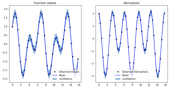
Model predictions are also similar to GP regression with only function values, butwe need more CG iterations to get accurate estimates of the predictive variance

# Set into eval mode
model.train()
model.eval()
likelihood.eval()

# Initialize plots
f, (y1_ax, y2_ax) = plt.subplots(1, 2, figsize=(12, 6))

# Make predictions
with torch.no_grad(), gpytorch.settings.max_cg_iterations(50):
    test_x = torch.linspace(lb, ub, 500)
    predictions = likelihood(model(test_x))
    mean = predictions.mean
    lower, upper = predictions.confidence_region()

# Plot training data as black stars
y1_ax.plot(train_x.detach().numpy(), train_y[:, 0].detach().numpy(), 'k*')
# Predictive mean as blue line
y1_ax.plot(test_x.numpy(), mean[:, 0].numpy(), 'b')
# Shade in confidence
y1_ax.fill_between(test_x.numpy(), lower[:, 0].numpy(), upper[:, 0].numpy(), alpha=0.5)
y1_ax.legend(['Observed Values', 'Mean', 'Confidence'])
y1_ax.set_title('Function values')

# Plot training data as black stars
y2_ax.plot(train_x.detach().numpy(), train_y[:, 1].detach().numpy(), 'k*')
# Predictive mean as blue line
y2_ax.plot(test_x.numpy(), mean[:, 1].numpy(), 'b')
# Shade in confidence
y2_ax.fill_between(test_x.numpy(), lower[:, 1].numpy(), upper[:, 1].numpy(), alpha=0.5)
y2_ax.legend(['Observed Derivatives', 'Mean', 'Confidence'])
y2_ax.set_title('Derivatives')

None