Exact GP Regression on Classification Labels

In this notebok, we demonstrate how one can convert classification problems into regression problems by performing fixed noise regression on the classification labels.

We follow the method of Dirichlet-based Gaussian Processes for Large-Scale Calibrated Classification who transform classification targets into regression ones by using an approximate likelihood.

import math
import torch
import numpy as np
import gpytorch
from matplotlib import pyplot as plt

%matplotlib inline
%load_ext autoreload
%autoreload 2

[pyKeOps]: Warning, no cuda detected. Switching to cpu only.

Generate Data

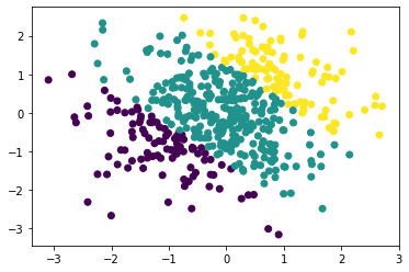
Firs, we will generate 500 data points from a smooth underlying latent function and have the inputs be iid Gaussian. The decision boundaries are given by rounding a latent function:

\(f(x,y) = \sin(0.15 \pi u + (x + y)) + 1,\) where \(u \sim \text{Unif}(0,1).\) Then, \(y = \text{round}(f(x,y)).\)

def gen_data(num_data, seed = 2019):
    torch.random.manual_seed(seed)

    x = torch.randn(num_data,1)
    y = torch.randn(num_data,1)

    u = torch.rand(1)
    data_fn = lambda x, y: 1 * torch.sin(0.15 * u * 3.1415 * (x + y)) + 1
    latent_fn = data_fn(x, y)
    z = torch.round(latent_fn).long().squeeze()
    return torch.cat((x,y),dim=1), z, data_fn

train_x, train_y, genfn = gen_data(500)

plt.scatter(train_x[:,0].numpy(), train_x[:,1].numpy(), c = train_y)

<matplotlib.collections.PathCollection at 0x7fe103195850>

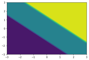
The below plots illustrate the decision boundary. We will predict the class logits and ultimately the predictions across \([-3, 3]^2\) for illustration; this region contains both interpolation and extrapolation.

test_d1 = np.linspace(-3, 3, 20)
test_d2 = np.linspace(-3, 3, 20)

test_x_mat, test_y_mat = np.meshgrid(test_d1, test_d2)
test_x_mat, test_y_mat = torch.Tensor(test_x_mat), torch.Tensor(test_y_mat)

test_x = torch.cat((test_x_mat.view(-1,1), test_y_mat.view(-1,1)),dim=1)
test_labels = torch.round(genfn(test_x_mat, test_y_mat))
test_y = test_labels.view(-1)

plt.contourf(test_x_mat.numpy(), test_y_mat.numpy(), test_labels.numpy())

<matplotlib.contour.QuadContourSet at 0x7fe1034378d0>

Setting Up the Model

The Dirichlet GP model is an exact GP model with a couple of caveats. First, it uses a special likelihood: a DirichletClassificationLikelihood, and second, it is natively a multi-output model (for each data point, we need to predict num_classes, \(C\), outputs) so we need to specify the batch shape for our mean and covariance functions.

The DirichletClassificationLikelhood is just a special type of FixedGaussianNoiseLikelihood that does the required data transformations into a regression problem for us. Succinctly, we soft one hot encode the labels into \(C\) outputs so that \(\alpha_i = \alpha_\epsilon\) if \(y_c=0\) and \(\alpha_i = 1 + \alpha_\epsilon\) if \(y_c=1.\) Then, our variances are \(\sigma^2 = \log(1./\alpha + 1.)\) and our targets are \(\log(\alpha) - 0.5 \sigma^2.\)

That is, rather than a classification problem, we have a regression problem with \(C\) outputs. For more details, please see the original paper.

from gpytorch.models import ExactGP
from gpytorch.likelihoods import DirichletClassificationLikelihood
from gpytorch.means import ConstantMean
from gpytorch.kernels import ScaleKernel, RBFKernel

# We will use the simplest form of GP model, exact inference
class DirichletGPModel(ExactGP):
    def __init__(self, train_x, train_y, likelihood, num_classes):
        super(DirichletGPModel, self).__init__(train_x, train_y, likelihood)
        self.mean_module = ConstantMean(batch_shape=torch.Size((num_classes,)))
        self.covar_module = ScaleKernel(
            RBFKernel(batch_shape=torch.Size((num_classes,))),
            batch_shape=torch.Size((num_classes,)),
        )

    def forward(self, x):
        mean_x = self.mean_module(x)
        covar_x = self.covar_module(x)
        return gpytorch.distributions.MultivariateNormal(mean_x, covar_x)

# initialize likelihood and model
# we let the DirichletClassificationLikelihood compute the targets for us
likelihood = DirichletClassificationLikelihood(train_y, learn_additional_noise=True)
model = DirichletGPModel(train_x, likelihood.transformed_targets, likelihood, num_classes=likelihood.num_classes)

Now we train and fit the model as we would any other GPyTorch model.

# this is for running the notebook in our testing framework
import os
smoke_test = ('CI' in os.environ)
training_iter = 2 if smoke_test else 50


# Find optimal model hyperparameters
model.train()
likelihood.train()

# Use the adam optimizer
optimizer = torch.optim.Adam(model.parameters(), lr=0.1)  # Includes GaussianLikelihood parameters

# "Loss" for GPs - the marginal log likelihood
mll = gpytorch.mlls.ExactMarginalLogLikelihood(likelihood, model)

for i in range(training_iter):
    # Zero gradients from previous iteration
    optimizer.zero_grad()
    # Output from model
    output = model(train_x)
    # Calc loss and backprop gradients
    loss = -mll(output, likelihood.transformed_targets).sum()
    loss.backward()
    if i % 5 == 0:
        print('Iter %d/%d - Loss: %.3f   lengthscale: %.3f   noise: %.3f' % (
            i + 1, training_iter, loss.item(),
            model.covar_module.base_kernel.lengthscale.mean().item(),
            model.likelihood.second_noise_covar.noise.mean().item()
        ))
    optimizer.step()

Iter 1/50 - Loss: 6.431   lengthscale: 0.693   noise: 0.693
Iter 6/50 - Loss: 5.934   lengthscale: 0.939   noise: 0.475
Iter 11/50 - Loss: 5.749   lengthscale: 1.056   noise: 0.322
Iter 16/50 - Loss: 5.591   lengthscale: 1.014   noise: 0.220
Iter 21/50 - Loss: 5.484   lengthscale: 0.906   noise: 0.153
Iter 26/50 - Loss: 5.391   lengthscale: 0.803   noise: 0.109
Iter 31/50 - Loss: 5.320   lengthscale: 0.722   noise: 0.080
Iter 36/50 - Loss: 5.282   lengthscale: 0.669   noise: 0.060
Iter 41/50 - Loss: 5.258   lengthscale: 0.632   noise: 0.047
Iter 46/50 - Loss: 5.237   lengthscale: 0.614   noise: 0.037

Model Predictions

model.eval()
likelihood.eval()

with gpytorch.settings.fast_pred_var(), torch.no_grad():
    test_dist = model(test_x)

    pred_means = test_dist.loc

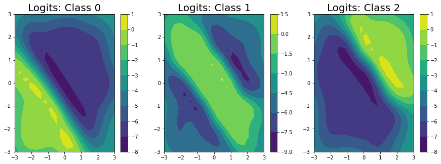
We’ve predicted the logits for each class in the classification problem, and can clearly see that the logits for class 0 are highest in the bottom left, the logits for class 2 are highest in the top right, and the logits for class 1 are highest in the middle.

fig, ax = plt.subplots(1, 3, figsize = (15, 5))

for i in range(3):
    im = ax[i].contourf(
        test_x_mat.numpy(), test_y_mat.numpy(), pred_means[i].numpy().reshape((20,20))
    )
    fig.colorbar(im, ax=ax[i])
    ax[i].set_title("Logits: Class " + str(i), fontsize = 20)

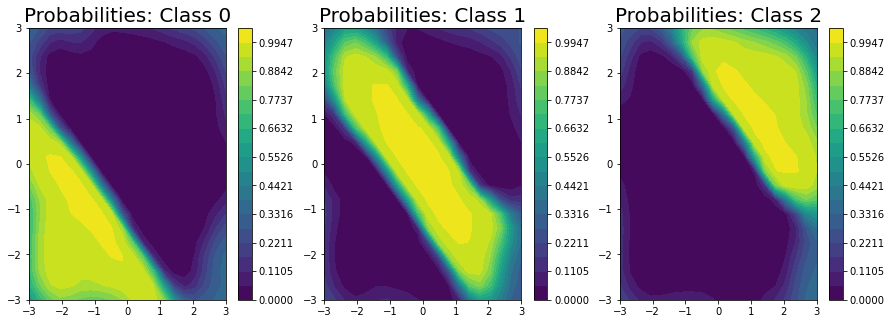
Unfortunately, we can’t get closed form estimates of the probabilities; however, we can approximate them with a lightweight sampling step using \(J\) samples from the posterior as:

\[\mathbb{E}(p(y_i = j)) = \int \frac{\exp\{f_i^*\}}{\sum_k^C \exp\{f_i^*\}} p(f^* | y) df^* \approx \frac{1}{J} \sum_j^J \frac{\exp\{f_{i,j}^*\}}{\sum_k^C \exp\{f_{i,j}^*\}}\]

Here, we draw \(256\) samples from the posterior.

pred_samples = test_dist.sample(torch.Size((256,))).exp()
probabilities = (pred_samples / pred_samples.sum(-2, keepdim=True)).mean(0)

/Users/wesleymaddox/anaconda3/lib/python3.7/site-packages/gpytorch/utils/cholesky.py:51: NumericalWarning: A not p.d., added jitter of 1.0e-05 to the diagonal
  warnings.warn(f"A not p.d., added jitter of {jitter_new:.1e} to the diagonal", NumericalWarning)

fig, ax = plt.subplots(1, 3, figsize = (15, 5))

levels = np.linspace(0, 1.05, 20)
for i in range(3):
    im = ax[i].contourf(
        test_x_mat.numpy(), test_y_mat.numpy(), probabilities[i].numpy().reshape((20,20)), levels=levels
    )
    fig.colorbar(im, ax=ax[i])
    ax[i].set_title("Probabilities: Class " + str(i), fontsize = 20)

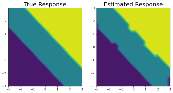
Finally, we plot the decision boundary (on the right) and the true decision boundary on the left. They align pretty closely.

To get the decision boundary from our model, all we need to do is to compute the elementwise maximium at each test point.

fig, ax = plt.subplots(1,2, figsize=(10, 5))

ax[0].contourf(test_x_mat.numpy(), test_y_mat.numpy(), test_labels.numpy())
ax[0].set_title('True Response', fontsize=20)

ax[1].contourf(test_x_mat.numpy(), test_y_mat.numpy(), pred_means.max(0)[1].reshape((20,20)))
ax[1].set_title('Estimated Response', fontsize=20)

Text(0.5, 1.0, 'Estimated Response')