[1]:
import tqdm
import math
import torch
import gpytorch
from matplotlib import pyplot as plt

# Make plots inline
%matplotlib inline
SVGP Model Updating
In this notebook, we will be describing a “fantasy model” strategy for stochastic variational GPs (SVGPs) analogous to fantasy modelling for exact GPs.
To understand what a “fantasy model” is, we first think about exact GPs. Imagine, we have trained a GP on some data \(\mathcal{D} := \{x_i, y_i\}_{i=1}^N\), which is the same as saying that \(\mathbf{y} \sim \mathcal{GP}(\mu(\mathbf{x}), K(\mathbf{x}, \mathbf{x}'))\).
If we observe some new data \(\mathcal{D}^*:= \{x_j, y_j\}_{j=1}^{N^*}\), then that data is easily incorporated into our GP model as \((\mathbf{y}, \mathbf{y}^*) \sim \mathcal{GP}(\mu([\mathbf{x}, \mathbf{x}^*]), K([\mathbf{x}, \mathbf{x}^*], [\mathbf{x}, \mathbf{x}^*]')\). To compute predictions with this new model (conditional on the same hyper-parameters), we could use the following piece of code for an exact GP:
updated_model = deepcopy(model)
updated_model.set_train_data(torch.cat((train_x, new_x)), torch.cat((train_y, new_y)), strict=False)
or we could take advantage of linear algebraic identies to efficiently produce the same model, which is the get_fantasy_model function for exact GPs in GPyTorch:
updated_model = model.get_fantasy_model(new_x, new_y)
The second approach is significantly more computationally efficient, costing \(\mathcal{O}((N^*)^2 N)\) time versus \(\mathcal{O}((N + N^*)^3)\) time.
In this tutorial notebook, we describe the online variational conditioning (OVC) approach of Maddox et al, ’21 which provides a closed form method for updating SVGPs in the same manner as exact GPs are updated with respect ot new data, via the usage of the get_fantasy_model method.
Training Data
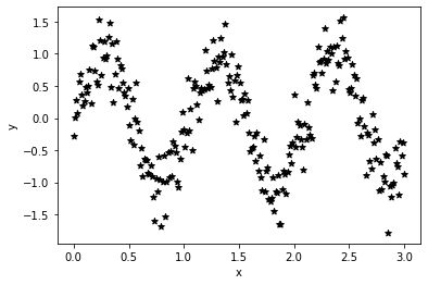
First, we construct some training data, here \(250\) data points from a noisy sine wave.
[2]:
train_x = torch.linspace(0, 3, 250).view(-1, 1).contiguous()
train_y = torch.sin(6. * train_x) + 0.3 * torch.randn_like(train_x)

plt.scatter(train_x, train_y, marker = "*", color = "black")
plt.xlabel("x")
plt.ylabel("y")
[2]:
Text(0, 0.5, 'y')
Model definition
Next, we define our model class definition. The only difference from a standard approximate GP is that we require the likelihood object to be a) Gaussian (for now) and b) to be stored inside of the ApproximateGP object.
[3]:
from gpytorch.models import ApproximateGP
from gpytorch.variational import CholeskyVariationalDistribution
from gpytorch.variational import VariationalStrategy

class GPModel(ApproximateGP):
    def __init__(self, inducing_points, likelihood):
        variational_distribution = CholeskyVariationalDistribution(inducing_points.size(0))
        variational_strategy = VariationalStrategy(self, inducing_points, variational_distribution, learn_inducing_locations=True)
        super(GPModel, self).__init__(variational_strategy)
        self.mean_module = gpytorch.means.ConstantMean()
        self.covar_module = gpytorch.kernels.ScaleKernel(gpytorch.kernels.RBFKernel())
        self.likelihood = likelihood

    def forward(self, x):
        mean_x = self.mean_module(x)
        covar_x = self.covar_module(x)
        return gpytorch.distributions.MultivariateNormal(mean_x, covar_x)
We initialize the SVGP with \(25\) inducing points.
[4]:
likelihood = gpytorch.likelihoods.GaussianLikelihood()
model = GPModel(torch.randn(25, 1) + 2., likelihood)
Model Training
As we don’t have a lot of data, we train the model with full-batch (although this isn’t a restriction) and for \(500\) iterations (b/c our choice of inducing points may not have been very good).
[5]:
model.train()
likelihood.train()

optimizer = torch.optim.Adam([
    {'params': model.parameters()},
    # {'params': likelihood.parameters()},
], lr=0.1)

# Our loss object. We're using the VariationalELBO
mll = gpytorch.mlls.VariationalELBO(likelihood, model, num_data=train_y.size(0))
[6]:
iters = 500 + 1

for i in range(iters):
    optimizer.zero_grad()
    output = model(train_x)
    loss = -mll(output, train_y.squeeze())
    loss.backward()
    optimizer.step()
    if i % 50 == 0:
        print("Iteration: ", i, "\t Loss:", loss.item())
Iteration:  0    Loss: 1.6754810810089111
Iteration:  50   Loss: 0.5079809427261353
Iteration:  100          Loss: 0.39197731018066406
Iteration:  150          Loss: 0.36815035343170166
Iteration:  200          Loss: 0.3656342625617981
Iteration:  250          Loss: 0.3653048574924469
Iteration:  300          Loss: 0.3654007315635681
Iteration:  350          Loss: 0.3680660128593445
Iteration:  400          Loss: 0.3646673262119293
Iteration:  450          Loss: 0.36463457345962524
Iteration:  500          Loss: 0.36551928520202637
Model Evaluation
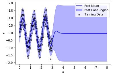
Now, that we’ve trained our SVGP, we choose some data to evaluate it on – here \(250\) data points from \([0, 8]\) to illustrate the performance both for interpolation (on \([0,3]\)) and extrapolation (on \([3, 8]\)).
[7]:
model.eval()
likelihood.eval()

test_x = torch.linspace(0, 8, 250).view(-1,1)
with torch.no_grad():
    posterior = likelihood(model(test_x))
As expected, the posterior model fits the training data well but reverts to a zero mean and high prediction outside of the region of the training data.
[9]:
plt.plot(test_x, posterior.mean, color = "blue", label = "Post Mean")
plt.fill_between(test_x.squeeze(), *posterior.confidence_region(), color = "blue", alpha = 0.3, label = "Post Conf Region")
plt.scatter(train_x, train_y, color = "black", marker = "*", alpha = 0.5, label = "Training Data")
plt.legend()
plt.xlabel("x")
plt.ylabel("y")
[9]:
Text(0, 0.5, 'y')
Model Updating
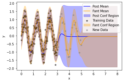
Now, we choose \(25\) points to condition the model on – imagining that these data points have just been acquired, perhaps from an active learning or Bayesian optimization loop.
[10]:
val_x = torch.linspace(3, 5, 25).view(-1,1)
val_y = torch.sin(6. * val_x) + 0.3 * torch.randn_like(val_x)
[11]:
cond_model = model.variational_strategy.get_fantasy_model(inputs=val_x, targets=val_y.squeeze())
/Users/wesleymaddox/Documents/GitHub/wjm_gpytorch/gpytorch/utils/cholesky.py:40: NumericalWarning: A not p.d., added jitter of 1.0e-06 to the diagonal
  warnings.warn(
/Users/wesleymaddox/Documents/GitHub/wjm_gpytorch/gpytorch/utils/cholesky.py:40: NumericalWarning: A not p.d., added jitter of 1.0e-05 to the diagonal
  warnings.warn(
/Users/wesleymaddox/Documents/GitHub/wjm_gpytorch/gpytorch/utils/cholesky.py:40: NumericalWarning: A not p.d., added jitter of 1.0e-04 to the diagonal
  warnings.warn(
Note that the updated model returned is an ExactGP class rather than a SVGP.
[12]:
cond_model
[12]:
_BaseExactGP(
  (likelihood): GaussianLikelihood(
    (noise_covar): HomoskedasticNoise(
      (raw_noise_constraint): GreaterThan(1.000E-04)
    )
  )
  (mean_module): ConstantMean()
  (covar_module): ScaleKernel(
    (base_kernel): RBFKernel(
      (raw_lengthscale_constraint): Positive()
      (distance_module): None
    )
    (raw_outputscale_constraint): Positive()
  )
)
We compute its posterior distribution on the same testing dataset as before.
[13]:
with torch.no_grad():
    updated_posterior = cond_model.likelihood(cond_model(test_x))
Finally, we plot the updated model, showing that the model has been updated to the newly observed data (grey) without forgetting the previous training data (black).
[15]:
plt.plot(test_x, posterior.mean, color = "blue", label = "Post Mean")
plt.fill_between(test_x.squeeze(), *posterior.confidence_region(), color = "blue", alpha = 0.3, label = "Post Conf Region")
plt.scatter(train_x, train_y, color = "black", marker = "*", alpha = 0.5, label = "Training Data")

plt.plot(test_x, updated_posterior.mean, color = "orange", label = "Fant Mean")
plt.fill_between(test_x.squeeze(), *updated_posterior.confidence_region(), color = "orange", alpha = 0.3, label = "Fant Conf Region")

plt.scatter(val_x, val_y, color = "grey", marker = "*", alpha = 0.5, label = "New Data")
plt.legend()
plt.xlabel("x")
plt.ylabel("y")
[15]:
Text(0, 0.5, 'y')
[ ]: