Spectral GP Learning with Deltas
In this paper, we demonstrate another approach to spectral learning with GPs, learning a spectral density as a simple mixture of deltas. This has been explored, for example, as early as Lázaro-Gredilla et al., 2010.
[1]:
import gpytorch
import torch
Load Data
For this notebook, we’ll be using a sample set of timeseries data of BART ridership on the 5 most commonly traveled stations in San Francisco. This subsample of data was selected and processed from Pyro’s examples http://docs.pyro.ai/en/stable/_modules/pyro/contrib/examples/bart.html
[2]:
import os
import urllib.request

smoke_test = ('CI' in os.environ)

if not smoke_test and not os.path.isfile('../BART_sample.pt'):
    print('Downloading \'BART\' sample dataset...')
    urllib.request.urlretrieve('https://drive.google.com/uc?export=download&id=1A6LqCHPA5lHa5S3lMH8mLMNEgeku8lRG', '../BART_sample.pt')
    torch.manual_seed(1)

if smoke_test:
    train_x, train_y, test_x, test_y = torch.randn(2, 100, 1), torch.randn(2, 100), torch.randn(2, 100, 1), torch.randn(2, 100)
else:
    train_x, train_y, test_x, test_y = torch.load('../BART_sample.pt', map_location='cpu')

if torch.cuda.is_available():
    train_x, train_y, test_x, test_y = train_x.cuda(), train_y.cuda(), test_x.cuda(), test_y.cuda()

print(train_x.shape, train_y.shape, test_x.shape, test_y.shape)
torch.Size([5, 1440, 1]) torch.Size([5, 1440]) torch.Size([5, 240, 1]) torch.Size([5, 240])
[3]:
train_x_min = train_x.min()
train_x_max = train_x.max()

train_x = train_x - train_x_min
test_x = test_x - train_x_min

train_y_mean = train_y.mean(dim=-1, keepdim=True)
train_y_std = train_y.std(dim=-1, keepdim=True)

train_y = (train_y - train_y_mean) / train_y_std

test_y = (test_y - train_y_mean) / train_y_std
Define a Model
The only thing of note here is the use of the kernel. For this example, we’ll learn a kernel with 2048 deltas in the mixture, and initialize by sampling directly from the empirical spectrum of the data.
[4]:
class SpectralDeltaGP(gpytorch.models.ExactGP):
    def __init__(self, train_x, train_y, num_deltas, noise_init=None):
        likelihood = gpytorch.likelihoods.GaussianLikelihood(noise_constraint=gpytorch.constraints.GreaterThan(1e-11))
        likelihood.register_prior("noise_prior", gpytorch.priors.HorseshoePrior(0.1), "noise")
        likelihood.noise = 1e-2

        super(SpectralDeltaGP, self).__init__(train_x, train_y, likelihood)
        self.mean_module = gpytorch.means.ConstantMean()
        base_covar_module = gpytorch.kernels.SpectralDeltaKernel(
            num_dims=train_x.size(-1),
            num_deltas=num_deltas,
        )
        base_covar_module.initialize_from_data(train_x[0], train_y[0])
        self.covar_module = gpytorch.kernels.ScaleKernel(base_covar_module)

    def forward(self, x):
        mean_x = self.mean_module(x)
        covar_x = self.covar_module(x)
        return gpytorch.distributions.MultivariateNormal(mean_x, covar_x)
[5]:
model = SpectralDeltaGP(train_x, train_y, num_deltas=1500)

if torch.cuda.is_available():
    model = model.cuda()
Train
[6]:
model.train()
mll = gpytorch.mlls.ExactMarginalLogLikelihood(model.likelihood, model)
optimizer = torch.optim.Adam(model.parameters(), lr=0.01)
scheduler = torch.optim.lr_scheduler.MultiStepLR(optimizer=optimizer, milestones=[40])

num_iters = 1000 if not smoke_test else 4

with gpytorch.settings.max_cholesky_size(0):  # Ensure we dont try to use Cholesky
    for i in range(num_iters):
        optimizer.zero_grad()
        output = model(train_x)
        loss = -mll(output, train_y)
        if train_x.dim() == 3:
            loss = loss.mean()
        loss.backward()
        optimizer.step()

        if i % 10 == 0:
            print(f'Iteration {i} - loss = {loss:.2f} - noise = {model.likelihood.noise.item():e}')

        scheduler.step()
Iteration 0 - loss = 24.75 - noise = 1.010000e-02
Iteration 10 - loss = 10.49 - noise = 1.107906e-02
Iteration 20 - loss = 3.68 - noise = 1.204213e-02
Iteration 30 - loss = 3.69 - noise = 1.276487e-02
Iteration 40 - loss = 2.00 - noise = 1.333853e-02
Iteration 50 - loss = 1.18 - noise = 1.337870e-02
Iteration 60 - loss = 1.10 - noise = 1.340098e-02
Iteration 70 - loss = 1.06 - noise = 1.341575e-02
Iteration 80 - loss = 1.05 - noise = 1.342753e-02
Iteration 90 - loss = 0.98 - noise = 1.343861e-02
Iteration 100 - loss = 0.98 - noise = 1.344975e-02
Iteration 110 - loss = 0.91 - noise = 1.346152e-02
Iteration 120 - loss = 0.94 - noise = 1.347341e-02
Iteration 130 - loss = 0.90 - noise = 1.348564e-02
Iteration 140 - loss = 0.78 - noise = 1.349751e-02
Iteration 150 - loss = 0.75 - noise = 1.350786e-02
Iteration 160 - loss = 0.75 - noise = 1.351690e-02
Iteration 170 - loss = 0.76 - noise = 1.352605e-02
Iteration 180 - loss = 0.74 - noise = 1.353530e-02
Iteration 190 - loss = 0.71 - noise = 1.354463e-02
Iteration 200 - loss = 0.71 - noise = 1.355418e-02
Iteration 210 - loss = 0.71 - noise = 1.356385e-02
Iteration 220 - loss = 0.71 - noise = 1.357375e-02
Iteration 230 - loss = 0.71 - noise = 1.358384e-02
Iteration 240 - loss = 0.70 - noise = 1.359454e-02
Iteration 250 - loss = 0.65 - noise = 1.360544e-02
Iteration 260 - loss = 0.69 - noise = 1.361629e-02
Iteration 270 - loss = 0.68 - noise = 1.362717e-02
Iteration 280 - loss = 0.67 - noise = 1.363807e-02
Iteration 290 - loss = 0.70 - noise = 1.364926e-02
Iteration 300 - loss = 0.70 - noise = 1.366061e-02
Iteration 310 - loss = 0.66 - noise = 1.367212e-02
Iteration 320 - loss = 0.65 - noise = 1.368315e-02
Iteration 330 - loss = 0.65 - noise = 1.369375e-02
Iteration 340 - loss = 0.64 - noise = 1.370386e-02
Iteration 350 - loss = 0.64 - noise = 1.371405e-02
Iteration 360 - loss = 0.62 - noise = 1.372444e-02
Iteration 370 - loss = 0.63 - noise = 1.373496e-02
Iteration 380 - loss = 0.63 - noise = 1.374584e-02
Iteration 390 - loss = 0.63 - noise = 1.375700e-02
Iteration 400 - loss = 0.63 - noise = 1.376797e-02
Iteration 410 - loss = 0.60 - noise = 1.377904e-02
Iteration 420 - loss = 0.61 - noise = 1.379027e-02
Iteration 430 - loss = 0.61 - noise = 1.380114e-02
Iteration 440 - loss = 0.62 - noise = 1.381227e-02
Iteration 450 - loss = 0.61 - noise = 1.382362e-02
Iteration 460 - loss = 0.58 - noise = 1.383517e-02
Iteration 470 - loss = 0.61 - noise = 1.384682e-02
Iteration 480 - loss = 0.63 - noise = 1.385889e-02
Iteration 490 - loss = 0.63 - noise = 1.387111e-02
Iteration 500 - loss = 0.61 - noise = 1.388358e-02
Iteration 510 - loss = 0.60 - noise = 1.389664e-02
Iteration 520 - loss = 0.60 - noise = 1.390998e-02
Iteration 530 - loss = 0.58 - noise = 1.392351e-02
Iteration 540 - loss = 0.62 - noise = 1.393629e-02
Iteration 550 - loss = 0.60 - noise = 1.394872e-02
Iteration 560 - loss = 0.60 - noise = 1.396085e-02
Iteration 570 - loss = 0.59 - noise = 1.397342e-02
Iteration 580 - loss = 0.63 - noise = 1.398654e-02
Iteration 590 - loss = 0.58 - noise = 1.400001e-02
Iteration 600 - loss = 0.58 - noise = 1.401340e-02
Iteration 610 - loss = 0.62 - noise = 1.402742e-02
Iteration 620 - loss = 0.59 - noise = 1.404199e-02
Iteration 630 - loss = 0.63 - noise = 1.405650e-02
Iteration 640 - loss = 0.63 - noise = 1.407137e-02
Iteration 650 - loss = 0.60 - noise = 1.408640e-02
Iteration 660 - loss = 0.58 - noise = 1.410100e-02
Iteration 670 - loss = 0.61 - noise = 1.411567e-02
Iteration 680 - loss = 0.59 - noise = 1.413125e-02
Iteration 690 - loss = 0.61 - noise = 1.414781e-02
Iteration 700 - loss = 0.58 - noise = 1.416490e-02
Iteration 710 - loss = 0.59 - noise = 1.418221e-02
Iteration 720 - loss = 0.59 - noise = 1.420006e-02
Iteration 730 - loss = 0.60 - noise = 1.421693e-02
Iteration 740 - loss = 0.59 - noise = 1.423384e-02
Iteration 750 - loss = 0.59 - noise = 1.424886e-02
Iteration 760 - loss = 0.59 - noise = 1.426466e-02
Iteration 770 - loss = 0.58 - noise = 1.428063e-02
Iteration 780 - loss = 0.60 - noise = 1.429628e-02
Iteration 790 - loss = 0.62 - noise = 1.431342e-02
Iteration 800 - loss = 0.57 - noise = 1.433162e-02
Iteration 810 - loss = 0.61 - noise = 1.435035e-02
Iteration 820 - loss = 0.57 - noise = 1.436906e-02
Iteration 830 - loss = 0.58 - noise = 1.438674e-02
Iteration 840 - loss = 0.58 - noise = 1.440415e-02
Iteration 850 - loss = 0.61 - noise = 1.442217e-02
Iteration 860 - loss = 0.58 - noise = 1.444128e-02
Iteration 870 - loss = 0.59 - noise = 1.445954e-02
Iteration 880 - loss = 0.61 - noise = 1.447739e-02
Iteration 890 - loss = 0.58 - noise = 1.449536e-02
Iteration 900 - loss = 0.54 - noise = 1.451268e-02
Iteration 910 - loss = 0.54 - noise = 1.452836e-02
Iteration 920 - loss = 0.55 - noise = 1.454423e-02
Iteration 930 - loss = 0.59 - noise = 1.456236e-02
Iteration 940 - loss = 0.56 - noise = 1.457988e-02
Iteration 950 - loss = 0.57 - noise = 1.459668e-02
Iteration 960 - loss = 0.56 - noise = 1.461400e-02
Iteration 970 - loss = 0.47 - noise = 1.462959e-02
Iteration 980 - loss = 0.47 - noise = 1.464033e-02
Iteration 990 - loss = 0.46 - noise = 1.464958e-02
[7]:
# Get into evaluation (predictive posterior) mode
model.eval()

# Test points are regularly spaced along [0,1]
# Make predictions by feeding model through likelihood
with torch.no_grad(), gpytorch.settings.max_cholesky_size(0), gpytorch.settings.fast_pred_var():
    test_x_f = torch.cat([train_x, test_x], dim=-2)
    observed_pred = model.likelihood(model(test_x_f))
    varz = observed_pred.variance
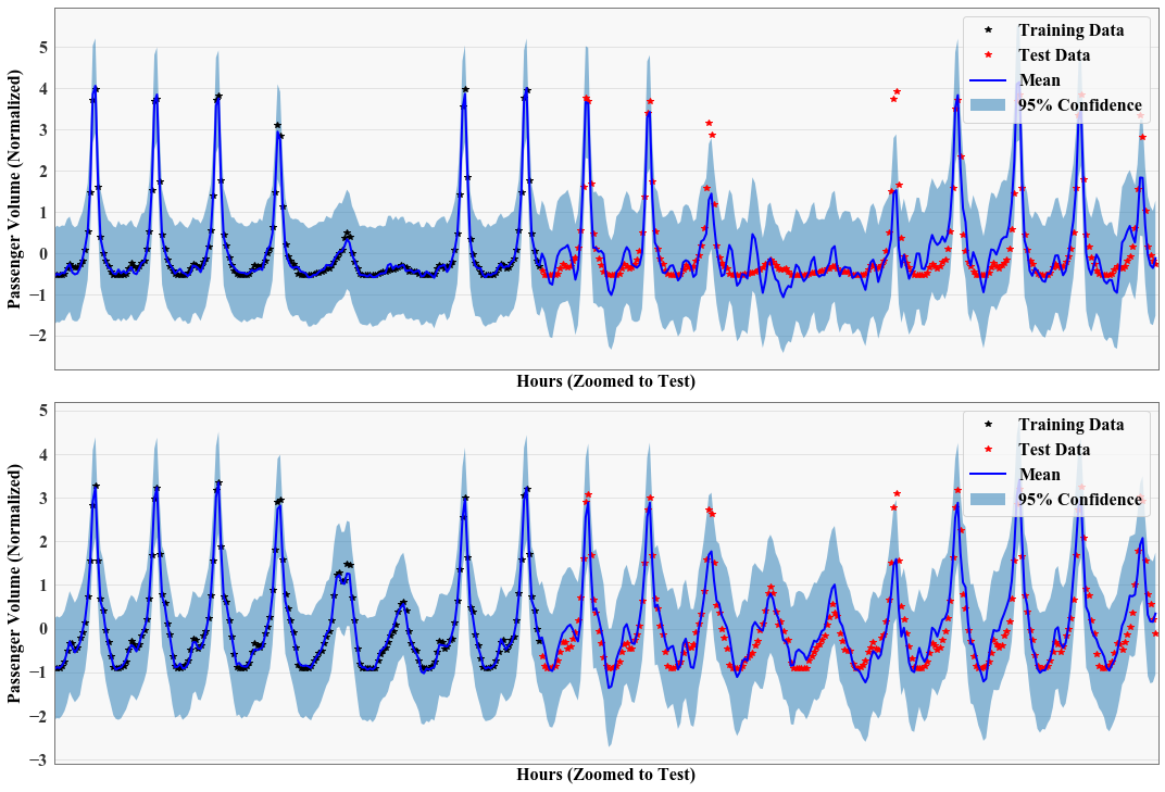
Plot Results
[8]:
from matplotlib import pyplot as plt

%matplotlib inline

_task = 3

plt.subplots(figsize=(15, 15), sharex=True, sharey=True)
for _task in range(2):
    ax = plt.subplot(3, 1, _task + 1)

    with torch.no_grad():
        # Initialize plot
#         f, ax = plt.subplots(1, 1, figsize=(16, 12))

        # Get upper and lower confidence bounds
        lower = observed_pred.mean - varz.sqrt() * 1.98
        upper = observed_pred.mean + varz.sqrt() * 1.98
        lower = lower[_task] #  + weight * test_x_f.squeeze()
        upper = upper[_task] # + weight * test_x_f.squeeze()

        # Plot training data as black stars
        ax.plot(train_x[_task].detach().cpu().numpy(), train_y[_task].detach().cpu().numpy(), 'k*')
        ax.plot(test_x[_task].detach().cpu().numpy(), test_y[_task].detach().cpu().numpy(), 'r*')
        # Plot predictive means as blue line
        ax.plot(test_x_f[_task].detach().cpu().numpy(), (observed_pred.mean[_task]).detach().cpu().numpy(), 'b')
        # Shade between the lower and upper confidence bounds
        ax.fill_between(test_x_f[_task].detach().cpu().squeeze().numpy(), lower.detach().cpu().numpy(), upper.detach().cpu().numpy(), alpha=0.5)
    #     ax.set_ylim([-3, 3])
        ax.legend(['Training Data', 'Test Data', 'Mean', '95% Confidence'], fontsize=16)
        ax.tick_params(axis='both', which='major', labelsize=16)
        ax.tick_params(axis='both', which='minor', labelsize=16)
        ax.set_ylabel('Passenger Volume (Normalized)', fontsize=16)
        ax.set_xlabel('Hours (Zoomed to Test)', fontsize=16)
        ax.set_xticks([])

        plt.xlim([1250, 1680])

plt.tight_layout()
[ ]: