Multitask GP Regression
Introduction
Multitask regression, introduced in this paper learns similarities in the outputs simultaneously. It’s useful when you are performing regression on multiple functions that share the same inputs, especially if they have similarities (such as being sinusodial).
Given inputs \(x\) and \(x'\), and tasks \(i\) and \(j\), the covariance between two datapoints and two tasks is given by
where \(k_\text{inputs}\) is a standard kernel (e.g. RBF) that operates on the inputs. \(k_\text{task}\) is a lookup table containing inter-task covariance.
[5]:
import math
import torch
import gpytorch
from matplotlib import pyplot as plt

%matplotlib inline
%load_ext autoreload
%autoreload 2
The autoreload extension is already loaded. To reload it, use:
  %reload_ext autoreload
Set up training data
In the next cell, we set up the training data for this example. We’ll be using 100 regularly spaced points on [0,1] which we evaluate the function on and add Gaussian noise to get the training labels.
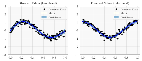
We’ll have two functions - a sine function (y1) and a cosine function (y2).
For MTGPs, our train_targets will actually have two dimensions: with the second dimension corresponding to the different tasks.
[6]:
train_x = torch.linspace(0, 1, 100)

train_y = torch.stack([
    torch.sin(train_x * (2 * math.pi)) + torch.randn(train_x.size()) * 0.2,
    torch.cos(train_x * (2 * math.pi)) + torch.randn(train_x.size()) * 0.2,
], -1)
Define a multitask model
The model should be somewhat similar to the ExactGP model in the simple regression example. The differences:
- We’re going to wrap ConstantMean with a
MultitaskMean. This makes sure we have a mean function for each task. - Rather than just using a RBFKernel, we’re using that in conjunction with a
MultitaskKernel. This gives us the covariance function described in the introduction. - We’re using a
MultitaskMultivariateNormalandMultitaskGaussianLikelihood. This allows us to deal with the predictions/outputs in a nice way. For example, when we call MultitaskMultivariateNormal.mean, we get an x num_tasksmatrix back.
You may also notice that we don’t use a ScaleKernel, since the MultitaskKernel will do some scaling for us. (This way we’re not overparameterizing the kernel.)
[9]:
class MultitaskGPModel(gpytorch.models.ExactGP):
    def __init__(self, train_x, train_y, likelihood):
        super(MultitaskGPModel, self).__init__(train_x, train_y, likelihood)
        self.mean_module = gpytorch.means.MultitaskMean(
            gpytorch.means.ConstantMean(), num_tasks=2
        )
        self.covar_module = gpytorch.kernels.MultitaskKernel(
            gpytorch.kernels.RBFKernel(), num_tasks=2, rank=1
        )

    def forward(self, x):
        mean_x = self.mean_module(x)
        covar_x = self.covar_module(x)
        return gpytorch.distributions.MultitaskMultivariateNormal(mean_x, covar_x)


likelihood = gpytorch.likelihoods.MultitaskGaussianLikelihood(num_tasks=2)
model = MultitaskGPModel(train_x, train_y, likelihood)
Train the model hyperparameters
[10]:
# this is for running the notebook in our testing framework
import os
smoke_test = ('CI' in os.environ)
training_iterations = 2 if smoke_test else 50


# Find optimal model hyperparameters
model.train()
likelihood.train()

# Use the adam optimizer
optimizer = torch.optim.Adam(model.parameters(), lr=0.1)  # Includes GaussianLikelihood parameters

# "Loss" for GPs - the marginal log likelihood
mll = gpytorch.mlls.ExactMarginalLogLikelihood(likelihood, model)

for i in range(training_iterations):
    optimizer.zero_grad()
    output = model(train_x)
    loss = -mll(output, train_y)
    loss.backward()
    print('Iter %d/%d - Loss: %.3f' % (i + 1, training_iterations, loss.item()))
    optimizer.step()
Iter 1/50 - Loss: 47.568
Iter 2/50 - Loss: 42.590
Iter 3/50 - Loss: 37.327
Iter 4/50 - Loss: 32.383
Iter 5/50 - Loss: 27.693
Iter 6/50 - Loss: 22.967
Iter 7/50 - Loss: 18.709
Iter 8/50 - Loss: 13.625
Iter 9/50 - Loss: 9.454
Iter 10/50 - Loss: 3.937
Iter 11/50 - Loss: -0.266
Iter 12/50 - Loss: -5.492
Iter 13/50 - Loss: -9.174
Iter 14/50 - Loss: -14.201
Iter 15/50 - Loss: -17.646
Iter 16/50 - Loss: -23.065
Iter 17/50 - Loss: -27.227
Iter 18/50 - Loss: -31.771
Iter 19/50 - Loss: -35.461
Iter 20/50 - Loss: -40.396
Iter 21/50 - Loss: -43.209
Iter 22/50 - Loss: -48.011
Iter 23/50 - Loss: -52.596
Iter 24/50 - Loss: -55.427
Iter 25/50 - Loss: -58.277
Iter 26/50 - Loss: -62.170
Iter 27/50 - Loss: -66.251
Iter 28/50 - Loss: -68.859
Iter 29/50 - Loss: -71.799
Iter 30/50 - Loss: -74.687
Iter 31/50 - Loss: -77.924
Iter 32/50 - Loss: -80.209
Iter 33/50 - Loss: -82.885
Iter 34/50 - Loss: -85.627
Iter 35/50 - Loss: -87.761
Iter 36/50 - Loss: -88.781
Iter 37/50 - Loss: -88.784
Iter 38/50 - Loss: -90.362
Iter 39/50 - Loss: -92.546
Iter 40/50 - Loss: -92.249
Iter 41/50 - Loss: -93.311
Iter 42/50 - Loss: -92.987
Iter 43/50 - Loss: -93.307
Iter 44/50 - Loss: -93.322
Iter 45/50 - Loss: -92.269
Iter 46/50 - Loss: -91.461
Iter 47/50 - Loss: -90.908
Iter 48/50 - Loss: -92.142
Iter 49/50 - Loss: -93.466
Iter 50/50 - Loss: -90.492
Make predictions with the model
[13]:
# Set into eval mode
model.eval()
likelihood.eval()

# Initialize plots
f, (y1_ax, y2_ax) = plt.subplots(1, 2, figsize=(8, 3))

# Make predictions
with torch.no_grad(), gpytorch.settings.fast_pred_var():
    test_x = torch.linspace(0, 1, 51)
    predictions = likelihood(model(test_x))
    mean = predictions.mean
    lower, upper = predictions.confidence_region()

# This contains predictions for both tasks, flattened out
# The first half of the predictions is for the first task
# The second half is for the second task

# Plot training data as black stars
y1_ax.plot(train_x.detach().numpy(), train_y[:, 0].detach().numpy(), 'k*')
# Predictive mean as blue line
y1_ax.plot(test_x.numpy(), mean[:, 0].numpy(), 'b')
# Shade in confidence
y1_ax.fill_between(test_x.numpy(), lower[:, 0].numpy(), upper[:, 0].numpy(), alpha=0.5)
y1_ax.set_ylim([-3, 3])
y1_ax.legend(['Observed Data', 'Mean', 'Confidence'])
y1_ax.set_title('Observed Values (Likelihood)')

# Plot training data as black stars
y2_ax.plot(train_x.detach().numpy(), train_y[:, 1].detach().numpy(), 'k*')
# Predictive mean as blue line
y2_ax.plot(test_x.numpy(), mean[:, 1].numpy(), 'b')
# Shade in confidence
y2_ax.fill_between(test_x.numpy(), lower[:, 1].numpy(), upper[:, 1].numpy(), alpha=0.5)
y2_ax.set_ylim([-3, 3])
y2_ax.legend(['Observed Data', 'Mean', 'Confidence'])
y2_ax.set_title('Observed Values (Likelihood)')

None
[ ]: