Batch Independent Multioutput GP
Introduction
This notebook demonstrates how to wrap independent GP models into a convenient Multi-Output GP model. It uses batch dimensions for efficient computation. Unlike in the Multitask GP Example, this do not model correlations between outcomes, but treats outcomes independently.
This type of model is useful if - when the number of training / test points is equal for the different outcomes - using the same covariance modules and / or likelihoods for each outcome
For non-block designs (i.e. when the above points do not apply), you should instead use a ModelList GP as described in the ModelList multioutput example.
[1]:
import math
import torch
import gpytorch
from matplotlib import pyplot as plt

%matplotlib inline
Set up training data
In the next cell, we set up the training data for this example. We’ll be using 100 regularly spaced points on [0,1] which we evaluate the function on and add Gaussian noise to get the training labels.
We’ll have two functions - a sine function (y1) and a cosine function (y2).
For MTGPs, our train_targets will actually have two dimensions: with the second dimension corresponding to the different tasks.
[2]:
train_x = torch.linspace(0, 1, 100)

train_y = torch.stack([
    torch.sin(train_x * (2 * math.pi)) + torch.randn(train_x.size()) * 0.2,
    torch.cos(train_x * (2 * math.pi)) + torch.randn(train_x.size()) * 0.2,
], -1)
Define a batch GP model
The model should be somewhat similar to the ExactGP model in the simple regression example. The differences:
- The model will use the batch dimension to learn multiple independent GPs simultaneously.
- We’re going to give the mean and covariance modules a
batch_shapeargument. This allows us to learn different hyperparameters for each model. - The model will return a
MultitaskMultivariateNormaldistribution rather than aMultivariateNormal. We will construct this distribution to convert the batch dimensions into distinct outputs.
[5]:
class BatchIndependentMultitaskGPModel(gpytorch.models.ExactGP):
    def __init__(self, train_x, train_y, likelihood):
        super().__init__(train_x, train_y, likelihood)
        self.mean_module = gpytorch.means.ConstantMean(batch_shape=torch.Size([2]))
        self.covar_module = gpytorch.kernels.ScaleKernel(
            gpytorch.kernels.RBFKernel(batch_shape=torch.Size([2])),
            batch_shape=torch.Size([2])
        )

    def forward(self, x):
        mean_x = self.mean_module(x)
        covar_x = self.covar_module(x)
        return gpytorch.distributions.MultitaskMultivariateNormal.from_batch_mvn(
            gpytorch.distributions.MultivariateNormal(mean_x, covar_x)
        )


likelihood = gpytorch.likelihoods.MultitaskGaussianLikelihood(num_tasks=2)
model = BatchIndependentMultitaskGPModel(train_x, train_y, likelihood)
Train the model hyperparameters
[6]:
# this is for running the notebook in our testing framework
import os
smoke_test = ('CI' in os.environ)
training_iterations = 2 if smoke_test else 50


# Find optimal model hyperparameters
model.train()
likelihood.train()

# Use the adam optimizer
optimizer = torch.optim.Adam(model.parameters(), lr=0.1)  # Includes GaussianLikelihood parameters

# "Loss" for GPs - the marginal log likelihood
mll = gpytorch.mlls.ExactMarginalLogLikelihood(likelihood, model)

for i in range(training_iterations):
    optimizer.zero_grad()
    output = model(train_x)
    loss = -mll(output, train_y)
    loss.backward()
    print('Iter %d/%d - Loss: %.3f' % (i + 1, training_iterations, loss.item()))
    optimizer.step()
Iter 1/50 - Loss: 122.929
Iter 2/50 - Loss: 119.192
Iter 3/50 - Loss: 115.233
Iter 4/50 - Loss: 111.096
Iter 5/50 - Loss: 106.824
Iter 6/50 - Loss: 102.458
Iter 7/50 - Loss: 98.038
Iter 8/50 - Loss: 93.608
Iter 9/50 - Loss: 89.226
Iter 10/50 - Loss: 84.959
Iter 11/50 - Loss: 80.849
Iter 12/50 - Loss: 76.895
Iter 13/50 - Loss: 73.049
Iter 14/50 - Loss: 69.255
Iter 15/50 - Loss: 65.470
Iter 16/50 - Loss: 61.671
Iter 17/50 - Loss: 57.848
Iter 18/50 - Loss: 54.001
Iter 19/50 - Loss: 50.137
Iter 20/50 - Loss: 46.268
Iter 21/50 - Loss: 42.412
Iter 22/50 - Loss: 38.591
Iter 23/50 - Loss: 34.830
Iter 24/50 - Loss: 31.155
Iter 25/50 - Loss: 27.596
Iter 26/50 - Loss: 24.183
Iter 27/50 - Loss: 20.947
Iter 28/50 - Loss: 17.915
Iter 29/50 - Loss: 15.109
Iter 30/50 - Loss: 12.543
Iter 31/50 - Loss: 10.213
Iter 32/50 - Loss: 8.110
Iter 33/50 - Loss: 6.225
Iter 34/50 - Loss: 4.556
Iter 35/50 - Loss: 3.111
Iter 36/50 - Loss: 1.903
Iter 37/50 - Loss: 0.948
Iter 38/50 - Loss: 0.252
Iter 39/50 - Loss: -0.192
Iter 40/50 - Loss: -0.410
Iter 41/50 - Loss: -0.438
Iter 42/50 - Loss: -0.323
Iter 43/50 - Loss: -0.113
Iter 44/50 - Loss: 0.145
Iter 45/50 - Loss: 0.410
Iter 46/50 - Loss: 0.648
Iter 47/50 - Loss: 0.836
Iter 48/50 - Loss: 0.961
Iter 49/50 - Loss: 1.016
Iter 50/50 - Loss: 1.004
Make predictions with the model
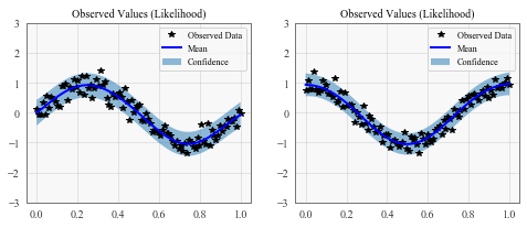
[7]:
# Set into eval mode
model.eval()
likelihood.eval()

# Initialize plots
f, (y1_ax, y2_ax) = plt.subplots(1, 2, figsize=(8, 3))

# Make predictions
with torch.no_grad(), gpytorch.settings.fast_pred_var():
    test_x = torch.linspace(0, 1, 51)
    predictions = likelihood(model(test_x))
    mean = predictions.mean
    lower, upper = predictions.confidence_region()

# This contains predictions for both tasks, flattened out
# The first half of the predictions is for the first task
# The second half is for the second task

# Plot training data as black stars
y1_ax.plot(train_x.detach().numpy(), train_y[:, 0].detach().numpy(), 'k*')
# Predictive mean as blue line
y1_ax.plot(test_x.numpy(), mean[:, 0].numpy(), 'b')
# Shade in confidence
y1_ax.fill_between(test_x.numpy(), lower[:, 0].numpy(), upper[:, 0].numpy(), alpha=0.5)
y1_ax.set_ylim([-3, 3])
y1_ax.legend(['Observed Data', 'Mean', 'Confidence'])
y1_ax.set_title('Observed Values (Likelihood)')

# Plot training data as black stars
y2_ax.plot(train_x.detach().numpy(), train_y[:, 1].detach().numpy(), 'k*')
# Predictive mean as blue line
y2_ax.plot(test_x.numpy(), mean[:, 1].numpy(), 'b')
# Shade in confidence
y2_ax.fill_between(test_x.numpy(), lower[:, 1].numpy(), upper[:, 1].numpy(), alpha=0.5)
y2_ax.set_ylim([-3, 3])
y2_ax.legend(['Observed Data', 'Mean', 'Confidence'])
y2_ax.set_title('Observed Values (Likelihood)')

None
[ ]: