Using Pòlya-Gamma Auxiliary Variables for Binary Classification
Overview
In this notebook, we’ll demonstrate how to use Pòlya-Gamma auxiliary variables to do efficient inference for Gaussian Process binary classification as in reference [1]. We will also use natural gradient descent, as described in more detail in the Natural gradient descent tutorial.
[1] Florian Wenzel, Theo Galy-Fajou, Christan Donner, Marius Kloft, Manfred Opper. Efficient Gaussian process classification using Pòlya-Gamma data augmentation. Proceedings of the AAAI Conference on Artificial Intelligence. 2019.
Pòlya-Gamma Augmentation
When a Gaussian Process prior is paired with a Gaussian likelihood inference can be done exactly with a simple closed form expression. Unfortunately this attractive feature does not carry over to non-conjugate likelihoods like the Bernoulli likelihood that arises in the context of binary classification with a logistic link function. Sampling-based stochastic variational inference offers a general strategy for dealing with non-conjugate likelihoods; see the corresponding tutorial.
Another possible strategy is to introduce additional latent variables that restore conjugacy. This is the strategy we follow here. In particular we are going to introduce a Pòlya-Gamma auxiliary variable for each data point in our training dataset. The Polya-Gamma distribution \(\rm{PG}\) is a univariate distribution with support on the positive real line. In our context it is interesting because if \(\omega_i\) is distributed according to \(\rm{PG}(1,0)\) then the logistic likelihood \(\sigma(\cdot)\) for data point \((x_i, y_i)\) can be represented as
\begin{align} \sigma(y_i f_i) = \frac{1}{1 + \exp(-y_i f_i)} = \tfrac{1}{2} \mathbb{E}_{\omega_i \sim \rm{PG}(1,0)} \left[ \exp \left(\tfrac{1}{2} y_i f_i - \tfrac{\omega_i}{2} f_i^2 \right) \right] \end{align}
where \(y_i \in \{-1, 1\}\) is the binary label of data point \(i\) and \(f_i\) is the Gaussian Process prior evaluated at input \(x_i\). The crucial point here is that \(f_i\) appears quadratically in the exponential within the expectation. In other words, conditioned on \(\omega_i\), we can integrate out \(f_i\) exactly, just as if we were doing regression with a Gaussian likelihood. For more details please see the original reference.
Setup
[1]:
import tqdm
import math
import torch
import gpytorch
from matplotlib import pyplot as plt

# Make plots inline
%matplotlib inline
For this example notebook, we’ll create a simple artificial dataset.
[2]:
import os
from math import floor

# this is for running the notebook in our testing framework
smoke_test = ('CI' in os.environ)

N = 100
X = torch.linspace(-1., 1., N)
probs = (torch.sin(X * math.pi).add(1.).div(2.))
y = torch.distributions.Bernoulli(probs=probs).sample()
X = X.unsqueeze(-1)

train_n = int(floor(0.8 * N))
indices = torch.randperm(N)
train_x = X[indices[:train_n]].contiguous()
train_y = y[indices[:train_n]].contiguous()

test_x = X[indices[train_n:]].contiguous()
test_y = y[indices[train_n:]].contiguous()

if torch.cuda.is_available():
    train_x, train_y, test_x, test_y = train_x.cuda(), train_y.cuda(), test_x.cuda(), test_y.cuda()
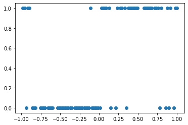
Let’s plot our artificial dataset. Note that here the binary labels are 0/1-valued; we will need to be careful to translate between this representation and the -1/1 representation that is most natural in the context of Pòlya-Gamma augementation.
[3]:
plt.plot(train_x.squeeze(-1).cpu(), train_y.cpu(), 'o')
[3]:
[<matplotlib.lines.Line2D at 0x7f7ee8dd4d90>]
The following steps create the dataloader objects. See the SVGP regression notebook for details.
[4]:
from torch.utils.data import TensorDataset, DataLoader

train_dataset = TensorDataset(train_x, train_y)
train_loader = DataLoader(train_dataset, batch_size=100000, shuffle=False)

test_dataset = TensorDataset(test_x, test_y)
test_loader = DataLoader(test_dataset, batch_size=1024, shuffle=False)
Variational Inference with PG Auxiliaries
We define a Bernoulli likelihood that leverages Pòlya-Gamma augmentation. It turns out that we can derive closed form updates for the Pòlya-Gamma auxiliary variables. To deal with the Gaussian Process we introduce inducing points and inducing locations. In particular we will need to learn a variational covariance matrix and a variational mean vector that control the inducing points. (See the discussion in the SVGP tutorial for more details.) We will use natural gradient updates to deal with these two variational parameters; this will allow us to take large steps, thus yielding fast convergence.
[5]:
class PGLikelihood(gpytorch.likelihoods._OneDimensionalLikelihood):
    # this method effectively computes the expected log likelihood
    # contribution to Eqn (10) in Reference [1].
    def expected_log_prob(self, target, input, *args, **kwargs):
        mean, variance = input.mean, input.variance
        # Compute the expectation E[f_i^2]
        raw_second_moment = variance + mean.pow(2)

        # Translate targets to be -1, 1
        target = target.to(mean.dtype).mul(2.).sub(1.)

        # We detach the following variable since we do not want
        # to differentiate through the closed-form PG update.
        c = raw_second_moment.detach().sqrt()
        # Compute mean of PG auxiliary variable omega: 0.5 * Expectation[omega]
        # See Eqn (11) and Appendix A2 and A3 in Reference [1] for details.
        half_omega = 0.25 * torch.tanh(0.5 * c) / c

        # Expected log likelihood
        res = 0.5 * target * mean - half_omega * raw_second_moment
        # Sum over data points in mini-batch
        res = res.sum(dim=-1)

        return res

    # define the likelihood
    def forward(self, function_samples):
        return torch.distributions.Bernoulli(logits=function_samples)

    # define the marginal likelihood using Gauss Hermite quadrature
    def marginal(self, function_dist):
        prob_lambda = lambda function_samples: self.forward(function_samples).probs
        probs = self.quadrature(prob_lambda, function_dist)
        return torch.distributions.Bernoulli(probs=probs)


# define the actual GP model (kernels, inducing points, etc.)
class GPModel(gpytorch.models.ApproximateGP):
    def __init__(self, inducing_points):
        variational_distribution = gpytorch.variational.NaturalVariationalDistribution(inducing_points.size(0))
        variational_strategy = gpytorch.variational.VariationalStrategy(
            self, inducing_points, variational_distribution, learn_inducing_locations=True
        )
        super(GPModel, self).__init__(variational_strategy)
        self.mean_module = gpytorch.means.ZeroMean()
        self.covar_module = gpytorch.kernels.ScaleKernel(gpytorch.kernels.RBFKernel())

    def forward(self, x):
        mean_x = self.mean_module(x)
        covar_x = self.covar_module(x)
        return gpytorch.distributions.MultivariateNormal(mean_x, covar_x)

# we initialize our model with M = 30 inducing points
M = 30
inducing_points = torch.linspace(-2., 2., M, dtype=train_x.dtype, device=train_x.device).unsqueeze(-1)
model = GPModel(inducing_points=inducing_points)
model.covar_module.base_kernel.initialize(lengthscale=0.2)
likelihood = PGLikelihood()

if torch.cuda.is_available():
    model = model.cuda()
    likelihood = likelihood.cuda()
Setup optimizers
We will use a NGD (Natural Gradient Descent) optimizer to deal with the inducing point covariance matrix and corresponding mean vector, while we will use the Adam optimizer for all other parameters (the kernel hyperparmaeters as well as the inducing point locations). Note that we use a pretty large learning rate for the NGD optimizer.
[6]:
variational_ngd_optimizer = gpytorch.optim.NGD(model.variational_parameters(), num_data=train_y.size(0), lr=0.1)

hyperparameter_optimizer = torch.optim.Adam([
    {'params': model.hyperparameters()},
    {'params': likelihood.parameters()},
], lr=0.01)
Define training loop
[7]:
model.train()
likelihood.train()
mll = gpytorch.mlls.VariationalELBO(likelihood, model, num_data=train_y.size(0))

num_epochs = 1 if smoke_test else 100
epochs_iter = tqdm.notebook.tqdm(range(num_epochs), desc="Epoch")
for i in epochs_iter:
    minibatch_iter = tqdm.notebook.tqdm(train_loader, desc="Minibatch", leave=False)

    for x_batch, y_batch in minibatch_iter:
        ### Perform NGD step to optimize variational parameters
        variational_ngd_optimizer.zero_grad()
        hyperparameter_optimizer.zero_grad()

        output = model(x_batch)
        loss = -mll(output, y_batch)
        minibatch_iter.set_postfix(loss=loss.item())
        loss.backward()
        variational_ngd_optimizer.step()
        hyperparameter_optimizer.step()
Visualization and Evaluation
[8]:
# push training data points through model
train_mean_f = model(train_x).loc.data.cpu()
# plot training data with y being -1/1 valued
plt.plot(train_x.squeeze(-1).cpu(), train_y.mul(2.).sub(1.).cpu(), 'o')
# plot mean gaussian process posterior mean evaluated at training data
plt.plot(train_x.squeeze(-1).cpu(), train_mean_f.cpu(), 'x')
[8]:
[<matplotlib.lines.Line2D at 0x7f7ee968da30>]
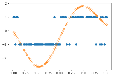
As expected the Gaussian Process posterior mean (plotted in orange) gives confident predictions in the regions where the correct label is unambiguous (e.g. for x ~ 0.5) and gives unconfident predictions in regions where the correct label is ambiguous (e.g. x ~ 0.0).
We compute the negative log likelihood (NLL) and classification accuracy on the held-out test data.
[9]:
model.eval()
likelihood.eval()
with torch.no_grad():
    nlls = -likelihood.log_marginal(test_y, model(test_x))
    acc = (likelihood(model(test_x)).probs.gt(0.5) == test_y.bool()).float().mean()
print('Test NLL: {:.4f}'.format(nlls.mean()))
print('Test Acc: {:.4f}'.format(acc.mean()))
Test NLL: 0.3481
Test Acc: 0.9000