Variational GPs w/ Multiple Outputs
Introduction
In this example, we will demonstrate how to construct approximate/variational GPs that can model vector-valued functions (e.g. multitask/multi-output GPs).
[1]:
import math
import torch
import gpytorch
import tqdm
from matplotlib import pyplot as plt

%matplotlib inline
%load_ext autoreload
%autoreload 2
Set up training data
In the next cell, we set up the training data for this example. We’ll be using 100 regularly spaced points on [0,1] which we evaluate the function on and add Gaussian noise to get the training labels.
We’ll have four functions - all of which are some sort of sinusoid. Our train_targets will actually have two dimensions: with the second dimension corresponding to the different tasks.
[2]:
train_x = torch.linspace(0, 1, 100)

train_y = torch.stack([
    torch.sin(train_x * (2 * math.pi)) + torch.randn(train_x.size()) * 0.2,
    torch.cos(train_x * (2 * math.pi)) + torch.randn(train_x.size()) * 0.2,
    torch.sin(train_x * (2 * math.pi)) + 2 * torch.cos(train_x * (2 * math.pi)) + torch.randn(train_x.size()) * 0.2,
    -torch.cos(train_x * (2 * math.pi)) + torch.randn(train_x.size()) * 0.2,
], -1)

print(train_x.shape, train_y.shape)
torch.Size([100]) torch.Size([100, 4])
Define a multitask model
We are going to construct a batch variational GP - using a CholeskyVariationalDistribution and a VariationalStrategy. Each of the batch dimensions is going to correspond to one of the outputs. In addition, we will wrap the variational strategy to make the output appear as a MultitaskMultivariateNormal distribution. Here are the changes that we’ll need to make:
- Our inducing points will need to have shape
2 x m x 1(wheremis the number of inducing points). This ensures that we learn a different set of inducing points for each output dimension. - The
CholeskyVariationalDistribution, mean module, and covariance modules will all need to include abatch_shape=torch.Size([2])argument. This ensures that we learn a different set of variational parameters and hyperparameters for each output dimension. - The
VariationalStrategyobject should be wrapped by a variational strategy that handles multitask models. We describe them below:
Types of Variational Multitask Models
The most general purpose multitask model is the Linear Model of Coregionalization (LMC), which assumes that each output dimension (task) is the linear combination of some latent functions \(\mathbf g(\cdot) = [g^{(1)}(\cdot), \ldots, g^{(Q)}(\cdot)]\):
where \(a^{(i)}\) are learnable parameters.
[3]:
num_latents = 3
num_tasks = 4

class MultitaskGPModel(gpytorch.models.ApproximateGP):
    def __init__(self):
        # Let's use a different set of inducing points for each latent function
        inducing_points = torch.rand(num_latents, 16, 1)

        # We have to mark the CholeskyVariationalDistribution as batch
        # so that we learn a variational distribution for each task
        variational_distribution = gpytorch.variational.CholeskyVariationalDistribution(
            inducing_points.size(-2), batch_shape=torch.Size([num_latents])
        )

        # We have to wrap the VariationalStrategy in a LMCVariationalStrategy
        # so that the output will be a MultitaskMultivariateNormal rather than a batch output
        variational_strategy = gpytorch.variational.LMCVariationalStrategy(
            gpytorch.variational.VariationalStrategy(
                self, inducing_points, variational_distribution, learn_inducing_locations=True
            ),
            num_tasks=4,
            num_latents=3,
            latent_dim=-1
        )

        super().__init__(variational_strategy)

        # The mean and covariance modules should be marked as batch
        # so we learn a different set of hyperparameters
        self.mean_module = gpytorch.means.ConstantMean(batch_shape=torch.Size([num_latents]))
        self.covar_module = gpytorch.kernels.ScaleKernel(
            gpytorch.kernels.RBFKernel(batch_shape=torch.Size([num_latents])),
            batch_shape=torch.Size([num_latents])
        )

    def forward(self, x):
        # The forward function should be written as if we were dealing with each output
        # dimension in batch
        mean_x = self.mean_module(x)
        covar_x = self.covar_module(x)
        return gpytorch.distributions.MultivariateNormal(mean_x, covar_x)


model = MultitaskGPModel()
likelihood = gpytorch.likelihoods.MultitaskGaussianLikelihood(num_tasks=num_tasks)
With all of the batch_shape arguments - it may look like we’re learning a batch of GPs. However, LMCVariationalStrategy objects convert this batch_dimension into a (non-batch) MultitaskMultivariateNormal.
[4]:
likelihood(model(train_x)).rsample().shape
[4]:
torch.Size([100, 4])
The LMC model allows there to be linear dependencies between outputs/tasks. Alternatively, if we want independent output dimensions, we can replace LMCVariationalStrategy with IndependentMultitaskVariationalStrategy:
[5]:
class IndependentMultitaskGPModel(gpytorch.models.ApproximateGP):
    def __init__(self):
        # Let's use a different set of inducing points for each task
        inducing_points = torch.rand(num_tasks, 16, 1)

        # We have to mark the CholeskyVariationalDistribution as batch
        # so that we learn a variational distribution for each task
        variational_distribution = gpytorch.variational.CholeskyVariationalDistribution(
            inducing_points.size(-2), batch_shape=torch.Size([num_tasks])
        )

        variational_strategy = gpytorch.variational.IndependentMultitaskVariationalStrategy(
            gpytorch.variational.VariationalStrategy(
                self, inducing_points, variational_distribution, learn_inducing_locations=True
            ),
            num_tasks=4,
        )

        super().__init__(variational_strategy)

        # The mean and covariance modules should be marked as batch
        # so we learn a different set of hyperparameters
        self.mean_module = gpytorch.means.ConstantMean(batch_shape=torch.Size([num_tasks]))
        self.covar_module = gpytorch.kernels.ScaleKernel(
            gpytorch.kernels.RBFKernel(batch_shape=torch.Size([num_tasks])),
            batch_shape=torch.Size([num_tasks])
        )

    def forward(self, x):
        # The forward function should be written as if we were dealing with each output
        # dimension in batch
        mean_x = self.mean_module(x)
        covar_x = self.covar_module(x)
        return gpytorch.distributions.MultivariateNormal(mean_x, covar_x)
Note that all the batch sizes for IndependentMultitaskVariationalStrategy are now num_tasks rather than num_latents.
Output modes
By default, LMCVariationalStrategy and IndependentMultitaskVariationalStrategy produce vector-valued outputs. In other words, they return a MultitaskMultivariateNormal distribution – containing all task values for each input.
This is similar to the ExactGP model described in the multitask GP regression tutorial.
[6]:
output = model(train_x)
print(output.__class__.__name__, output.event_shape)
MultitaskMultivariateNormal torch.Size([100, 4])
Alternatively, if each input is only associated with a single task, passing in the task_indices argument will specify which task to return for each input. The result will be a standard MultivariateNormal distribution – where each output corresponds to each input’s specified task.
This is similar to the ExactGP model described in the Hadamard multitask GP regression tutorial
[7]:
x = train_x[..., :5]
task_indices = torch.LongTensor([0, 1, 3, 2, 2])
output = model(x, task_indices=task_indices)
print(output.__class__.__name__, output.event_shape)
MultivariateNormal torch.Size([5])
Train the model
This code should look similar to the SVGP training code
[8]:
# this is for running the notebook in our testing framework
import os
smoke_test = ('CI' in os.environ)
num_epochs = 1 if smoke_test else 500


model.train()
likelihood.train()

optimizer = torch.optim.Adam([
    {'params': model.parameters()},
    {'params': likelihood.parameters()},
], lr=0.1)

# Our loss object. We're using the VariationalELBO, which essentially just computes the ELBO
mll = gpytorch.mlls.VariationalELBO(likelihood, model, num_data=train_y.size(0))

# We use more CG iterations here because the preconditioner introduced in the NeurIPS paper seems to be less
# effective for VI.
epochs_iter = tqdm.tqdm_notebook(range(num_epochs), desc="Epoch")
for i in epochs_iter:
    # Within each iteration, we will go over each minibatch of data
    optimizer.zero_grad()
    output = model(train_x)
    loss = -mll(output, train_y)
    epochs_iter.set_postfix(loss=loss.item())
    loss.backward()
    optimizer.step()
/home/gpleiss/miniconda3/envs/gpytorch/lib/python3.7/site-packages/ipykernel_launcher.py:20: TqdmDeprecationWarning: This function will be removed in tqdm==5.0.0
Please use `tqdm.notebook.tqdm` instead of `tqdm.tqdm_notebook`
Make predictions with the model
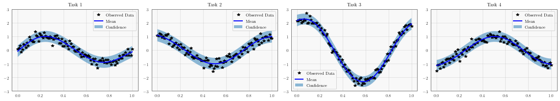
[9]:
# Set into eval mode
model.eval()
likelihood.eval()

# Initialize plots
fig, axs = plt.subplots(1, num_tasks, figsize=(4 * num_tasks, 3))

# Make predictions
with torch.no_grad(), gpytorch.settings.fast_pred_var():
    test_x = torch.linspace(0, 1, 51)
    predictions = likelihood(model(test_x))
    mean = predictions.mean
    lower, upper = predictions.confidence_region()

for task, ax in enumerate(axs):
    # Plot training data as black stars
    ax.plot(train_x.detach().numpy(), train_y[:, task].detach().numpy(), 'k*')
    # Predictive mean as blue line
    ax.plot(test_x.numpy(), mean[:, task].numpy(), 'b')
    # Shade in confidence
    ax.fill_between(test_x.numpy(), lower[:, task].numpy(), upper[:, task].numpy(), alpha=0.5)
    ax.set_ylim([-3, 3])
    ax.legend(['Observed Data', 'Mean', 'Confidence'])
    ax.set_title(f'Task {task + 1}')

fig.tight_layout()
None