GPyTorch Regression Tutorial
Introduction
In this notebook, we demonstrate many of the design features of GPyTorch using the simplest example, training an RBF kernel Gaussian process on a simple function. We’ll be modeling the function
with 100 training examples, and testing on 51 test examples.
Note: this notebook is not necessarily intended to teach the mathematical background of Gaussian processes, but rather how to train a simple one and make predictions in GPyTorch. For a mathematical treatment, Chapter 2 of Gaussian Processes for Machine Learning provides a very thorough introduction to GP regression (this entire text is highly recommended): http://www.gaussianprocess.org/gpml/chapters/RW2.pdf
[7]:
import math
import torch
import gpytorch
from matplotlib import pyplot as plt

%matplotlib inline
%load_ext autoreload
%autoreload 2
The autoreload extension is already loaded. To reload it, use:
  %reload_ext autoreload
Set up training data
In the next cell, we set up the training data for this example. We’ll be using 100 regularly spaced points on [0,1] which we evaluate the function on and add Gaussian noise to get the training labels.
[8]:
# Training data is 100 points in [0,1] inclusive regularly spaced
train_x = torch.linspace(0, 1, 100)
# True function is sin(2*pi*x) with Gaussian noise
train_y = torch.sin(train_x * (2 * math.pi)) + torch.randn(train_x.size()) * math.sqrt(0.04)
Setting up the model
The next cell demonstrates the most critical features of a user-defined Gaussian process model in GPyTorch. Building a GP model in GPyTorch is different in a number of ways.
First in contrast to many existing GP packages, we do not provide full GP models for the user. Rather, we provide the tools necessary to quickly construct one. This is because we believe, analogous to building a neural network in standard PyTorch, it is important to have the flexibility to include whatever components are necessary. As can be seen in more complicated examples, this allows the user great flexibility in designing custom models.
For most GP regression models, you will need to construct the following GPyTorch objects:
- A GP Model (
gpytorch.models.ExactGP) - This handles most of the inference. - A Likelihood (
gpytorch.likelihoods.GaussianLikelihood) - This is the most common likelihood used for GP regression. - A Mean - This defines the prior mean of the GP.(If you don’t know which mean to use, a
gpytorch.means.ConstantMean()is a good place to start.) - A Kernel - This defines the prior covariance of the GP.(If you don’t know which kernel to use, a
gpytorch.kernels.ScaleKernel(gpytorch.kernels.RBFKernel())is a good place to start). - A MultivariateNormal Distribution (
gpytorch.distributions.MultivariateNormal) - This is the object used to represent multivariate normal distributions.
The GP Model
The components of a user built (Exact, i.e. non-variational) GP model in GPyTorch are, broadly speaking:
- An
__init__method that takes the training data and a likelihood, and constructs whatever objects are necessary for the model’sforwardmethod. This will most commonly include things like a mean module and a kernel module. - A
forwardmethod that takes in some \(n \times d\) dataxand returns aMultivariateNormalwith the prior mean and covariance evaluated atx. In other words, we return the vector \(\mu(x)\) and the \(n \times n\) matrix \(K_{xx}\) representing the prior mean and covariance matrix of the GP.
This specification leaves a large amount of flexibility when defining a model. For example, to compose two kernels via addition, you can either add the kernel modules directly:
self.covar_module = ScaleKernel(RBFKernel() + LinearKernel())
Or you can add the outputs of the kernel in the forward method:
covar_x = self.rbf_kernel_module(x) + self.white_noise_module(x)
The likelihood
The simplest likelihood for regression is the gpytorch.likelihoods.GaussianLikelihood. This assumes a homoskedastic noise model (i.e. all inputs have the same observational noise).
There are other options for exact GP regression, such as the FixedNoiseGaussianLikelihood, which assigns a different observed noise value to different training inputs.
[9]:
# We will use the simplest form of GP model, exact inference
class ExactGPModel(gpytorch.models.ExactGP):
    def __init__(self, train_x, train_y, likelihood):
        super(ExactGPModel, self).__init__(train_x, train_y, likelihood)
        self.mean_module = gpytorch.means.ConstantMean()
        self.covar_module = gpytorch.kernels.ScaleKernel(gpytorch.kernels.RBFKernel())

    def forward(self, x):
        mean_x = self.mean_module(x)
        covar_x = self.covar_module(x)
        return gpytorch.distributions.MultivariateNormal(mean_x, covar_x)

# initialize likelihood and model
likelihood = gpytorch.likelihoods.GaussianLikelihood()
model = ExactGPModel(train_x, train_y, likelihood)
Model modes
Like most PyTorch modules, the ExactGP has a .train() and .eval() mode. - .train() mode is for optimizing model hyperameters. - .eval() mode is for computing predictions through the model posterior.
Training the model
In the next cell, we handle using Type-II MLE to train the hyperparameters of the Gaussian process.
The most obvious difference here compared to many other GP implementations is that, as in standard PyTorch, the core training loop is written by the user. In GPyTorch, we make use of the standard PyTorch optimizers as from torch.optim, and all trainable parameters of the model should be of type torch.nn.Parameter. Because GP models directly extend torch.nn.Module, calls to methods like model.parameters() or model.named_parameters() function as you might expect coming from
PyTorch.
In most cases, the boilerplate code below will work well. It has the same basic components as the standard PyTorch training loop:
- Zero all parameter gradients
- Call the model and compute the loss
- Call backward on the loss to fill in gradients
- Take a step on the optimizer
However, defining custom training loops allows for greater flexibility. For example, it is easy to save the parameters at each step of training, or use different learning rates for different parameters (which may be useful in deep kernel learning for example).
[10]:
# this is for running the notebook in our testing framework
import os
smoke_test = ('CI' in os.environ)
training_iter = 2 if smoke_test else 50


# Find optimal model hyperparameters
model.train()
likelihood.train()

# Use the adam optimizer
optimizer = torch.optim.Adam(model.parameters(), lr=0.1)  # Includes GaussianLikelihood parameters

# "Loss" for GPs - the marginal log likelihood
mll = gpytorch.mlls.ExactMarginalLogLikelihood(likelihood, model)

for i in range(training_iter):
    # Zero gradients from previous iteration
    optimizer.zero_grad()
    # Output from model
    output = model(train_x)
    # Calc loss and backprop gradients
    loss = -mll(output, train_y)
    loss.backward()
    print('Iter %d/%d - Loss: %.3f   lengthscale: %.3f   noise: %.3f' % (
        i + 1, training_iter, loss.item(),
        model.covar_module.base_kernel.lengthscale.item(),
        model.likelihood.noise.item()
    ))
    optimizer.step()
Iter 1/50 - Loss: 0.939   lengthscale: 0.693   noise: 0.693
Iter 2/50 - Loss: 0.908   lengthscale: 0.644   noise: 0.644
Iter 3/50 - Loss: 0.874   lengthscale: 0.598   noise: 0.598
Iter 4/50 - Loss: 0.837   lengthscale: 0.555   noise: 0.554
Iter 5/50 - Loss: 0.795   lengthscale: 0.514   noise: 0.513
Iter 6/50 - Loss: 0.749   lengthscale: 0.476   noise: 0.474
Iter 7/50 - Loss: 0.699   lengthscale: 0.440   noise: 0.437
Iter 8/50 - Loss: 0.649   lengthscale: 0.405   noise: 0.402
Iter 9/50 - Loss: 0.600   lengthscale: 0.372   noise: 0.369
Iter 10/50 - Loss: 0.556   lengthscale: 0.342   noise: 0.339
Iter 11/50 - Loss: 0.516   lengthscale: 0.315   noise: 0.310
Iter 12/50 - Loss: 0.480   lengthscale: 0.291   noise: 0.284
Iter 13/50 - Loss: 0.448   lengthscale: 0.270   noise: 0.259
Iter 14/50 - Loss: 0.413   lengthscale: 0.254   noise: 0.237
Iter 15/50 - Loss: 0.380   lengthscale: 0.241   noise: 0.216
Iter 16/50 - Loss: 0.355   lengthscale: 0.231   noise: 0.197
Iter 17/50 - Loss: 0.314   lengthscale: 0.223   noise: 0.179
Iter 18/50 - Loss: 0.292   lengthscale: 0.218   noise: 0.163
Iter 19/50 - Loss: 0.262   lengthscale: 0.214   noise: 0.148
Iter 20/50 - Loss: 0.236   lengthscale: 0.214   noise: 0.135
Iter 21/50 - Loss: 0.201   lengthscale: 0.216   noise: 0.122
Iter 22/50 - Loss: 0.176   lengthscale: 0.220   noise: 0.111
Iter 23/50 - Loss: 0.158   lengthscale: 0.224   noise: 0.102
Iter 24/50 - Loss: 0.125   lengthscale: 0.231   noise: 0.093
Iter 25/50 - Loss: 0.101   lengthscale: 0.239   noise: 0.085
Iter 26/50 - Loss: 0.078   lengthscale: 0.247   noise: 0.077
Iter 27/50 - Loss: 0.066   lengthscale: 0.256   noise: 0.071
Iter 28/50 - Loss: 0.052   lengthscale: 0.265   noise: 0.065
Iter 29/50 - Loss: 0.036   lengthscale: 0.276   noise: 0.060
Iter 30/50 - Loss: 0.036   lengthscale: 0.286   noise: 0.056
Iter 31/50 - Loss: 0.031   lengthscale: 0.297   noise: 0.052
Iter 32/50 - Loss: 0.028   lengthscale: 0.306   noise: 0.048
Iter 33/50 - Loss: 0.030   lengthscale: 0.315   noise: 0.045
Iter 34/50 - Loss: 0.035   lengthscale: 0.322   noise: 0.043
Iter 35/50 - Loss: 0.039   lengthscale: 0.326   noise: 0.041
Iter 36/50 - Loss: 0.043   lengthscale: 0.329   noise: 0.039
Iter 37/50 - Loss: 0.047   lengthscale: 0.327   noise: 0.038
Iter 38/50 - Loss: 0.052   lengthscale: 0.323   noise: 0.037
Iter 39/50 - Loss: 0.048   lengthscale: 0.317   noise: 0.036
Iter 40/50 - Loss: 0.051   lengthscale: 0.309   noise: 0.036
Iter 41/50 - Loss: 0.051   lengthscale: 0.302   noise: 0.036
Iter 42/50 - Loss: 0.047   lengthscale: 0.295   noise: 0.036
Iter 43/50 - Loss: 0.048   lengthscale: 0.288   noise: 0.036
Iter 44/50 - Loss: 0.047   lengthscale: 0.281   noise: 0.037
Iter 45/50 - Loss: 0.047   lengthscale: 0.276   noise: 0.037
Iter 46/50 - Loss: 0.040   lengthscale: 0.273   noise: 0.038
Iter 47/50 - Loss: 0.037   lengthscale: 0.271   noise: 0.039
Iter 48/50 - Loss: 0.040   lengthscale: 0.270   noise: 0.040
Iter 49/50 - Loss: 0.033   lengthscale: 0.269   noise: 0.042
Iter 50/50 - Loss: 0.032   lengthscale: 0.269   noise: 0.043
Make predictions with the model
In the next cell, we make predictions with the model. To do this, we simply put the model and likelihood in eval mode, and call both modules on the test data.
Just as a user defined GP model returns a MultivariateNormal containing the prior mean and covariance from forward, a trained GP model in eval mode returns a MultivariateNormal containing the posterior mean and covariance. Thus, getting the predictive mean and variance, and then sampling functions from the GP at the given test points could be accomplished with calls like:
f_preds = model(test_x)
y_preds = likelihood(model(test_x))

f_mean = f_preds.mean
f_var = f_preds.variance
f_covar = f_preds.covariance_matrix
f_samples = f_preds.sample(sample_shape=torch.Size(1000,))
The gpytorch.settings.fast_pred_var context is not needed, but here we are giving a preview of using one of our cool features, getting faster predictive distributions using LOVE.
[11]:
# Get into evaluation (predictive posterior) mode
model.eval()
likelihood.eval()

# Test points are regularly spaced along [0,1]
# Make predictions by feeding model through likelihood
with torch.no_grad(), gpytorch.settings.fast_pred_var():
    test_x = torch.linspace(0, 1, 51)
    observed_pred = likelihood(model(test_x))
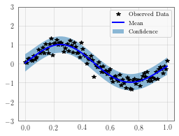
Plot the model fit
In the next cell, we plot the mean and confidence region of the Gaussian process model. The confidence_region method is a helper method that returns 2 standard deviations above and below the mean.
[12]:
with torch.no_grad():
    # Initialize plot
    f, ax = plt.subplots(1, 1, figsize=(4, 3))

    # Get upper and lower confidence bounds
    lower, upper = observed_pred.confidence_region()
    # Plot training data as black stars
    ax.plot(train_x.numpy(), train_y.numpy(), 'k*')
    # Plot predictive means as blue line
    ax.plot(test_x.numpy(), observed_pred.mean.numpy(), 'b')
    # Shade between the lower and upper confidence bounds
    ax.fill_between(test_x.numpy(), lower.numpy(), upper.numpy(), alpha=0.5)
    ax.set_ylim([-3, 3])
    ax.legend(['Observed Data', 'Mean', 'Confidence'])
[ ]: