Hadamard Multitask GP Regression
Introduction
This notebook demonstrates how to perform “Hadamard” multitask regression. This differs from the multitask gp regression example notebook in one key way:
- Here, we assume that we have observations for one task per input. For each input, we specify the task of the input that we observe. (The kernel that we learn is expressed as a Hadamard product of an input kernel and a task kernel)
- In the other notebook, we assume that we observe all tasks per input. (The kernel in that notebook is the Kronecker product of an input kernel and a task kernel).
Multitask regression, first introduced in this paper learns similarities in the outputs simultaneously. It’s useful when you are performing regression on multiple functions that share the same inputs, especially if they have similarities (such as being sinusodial).
Given inputs \(x\) and \(x'\), and tasks \(i\) and \(j\), the covariance between two datapoints and two tasks is given by
where \(k_\text{inputs}\) is a standard kernel (e.g. RBF) that operates on the inputs. \(k_\text{task}\) is a special kernel - the IndexKernel - which is a lookup table containing inter-task covariance.
[1]:
import math
import torch
import gpytorch
from matplotlib import pyplot as plt

%matplotlib inline
%load_ext autoreload
%autoreload 2
Set up training data
In the next cell, we set up the training data for this example. For each task we’ll be using 50 random points on [0,1), which we evaluate the function on and add Gaussian noise to get the training labels. Note that different inputs are used for each task.
We’ll have two functions - a sine function (y1) and a cosine function (y2).
[2]:
train_x1 = torch.rand(2000)
train_x2 = torch.rand(2000)

train_y1 = torch.sin(train_x1 * (2 * math.pi)) + torch.randn(train_x1.size()) * 0.2
train_y2 = torch.cos(train_x2 * (2 * math.pi)) + torch.randn(train_x2.size()) * 0.2
Set up a Hadamard multitask model
The model should be somewhat similar to the ExactGP model in the simple regression example.
The differences:
- The model takes two input: the inputs (x) and indices. The indices indicate which task the observation is for.
- Rather than just using a RBFKernel, we’re using that in conjunction with a IndexKernel.
- We don’t use a ScaleKernel, since the IndexKernel will do some scaling for us. (This way we’re not overparameterizing the kernel.)
[3]:
class MultitaskGPModel(gpytorch.models.ExactGP):
    def __init__(self, train_x, train_y, likelihood):
        super(MultitaskGPModel, self).__init__(train_x, train_y, likelihood)
        self.mean_module = gpytorch.means.ConstantMean()
        self.covar_module = gpytorch.kernels.RBFKernel()

        # We learn an IndexKernel for 2 tasks
        # (so we'll actually learn 2x2=4 tasks with correlations)
        self.task_covar_module = gpytorch.kernels.IndexKernel(num_tasks=2, rank=1)

    def forward(self,x,i):
        mean_x = self.mean_module(x)

        # Get input-input covariance
        covar_x = self.covar_module(x)
        # Get task-task covariance
        covar_i = self.task_covar_module(i)
        # Multiply the two together to get the covariance we want
        covar = covar_x.mul(covar_i)

        return gpytorch.distributions.MultivariateNormal(mean_x, covar)

likelihood = gpytorch.likelihoods.GaussianLikelihood()

train_i_task1 = torch.full((train_x1.shape[0],1), dtype=torch.long, fill_value=0)
train_i_task2 = torch.full((train_x2.shape[0],1), dtype=torch.long, fill_value=1)

full_train_x = torch.cat([train_x1, train_x2])
full_train_i = torch.cat([train_i_task1, train_i_task2])
full_train_y = torch.cat([train_y1, train_y2])

# Here we have two iterms that we're passing in as train_inputs
model = MultitaskGPModel((full_train_x, full_train_i), full_train_y, likelihood)
Training the model
In the next cell, we handle using Type-II MLE to train the hyperparameters of the Gaussian process.
See the simple regression example for more info on this step.
[4]:
# this is for running the notebook in our testing framework
import os
smoke_test = ('CI' in os.environ)
training_iterations = 2 if smoke_test else 50


# Find optimal model hyperparameters
model.train()
likelihood.train()

# Use the adam optimizer
optimizer = torch.optim.Adam(model.parameters(), lr=0.1)  # Includes GaussianLikelihood parameters

# "Loss" for GPs - the marginal log likelihood
mll = gpytorch.mlls.ExactMarginalLogLikelihood(likelihood, model)

for i in range(training_iterations):
    optimizer.zero_grad()
    output = model(full_train_x, full_train_i)
    loss = -mll(output, full_train_y)
    loss.backward()
    print('Iter %d/50 - Loss: %.3f' % (i + 1, loss.item()))
    optimizer.step()
Iter 1/50 - Loss: 1.000
Iter 2/50 - Loss: 0.960
Iter 3/50 - Loss: 0.918
Iter 4/50 - Loss: 0.874
Iter 5/50 - Loss: 0.831
Iter 6/50 - Loss: 0.788
Iter 7/50 - Loss: 0.745
Iter 8/50 - Loss: 0.702
Iter 9/50 - Loss: 0.659
Iter 10/50 - Loss: 0.618
Iter 11/50 - Loss: 0.580
Iter 12/50 - Loss: 0.545
Iter 13/50 - Loss: 0.511
Iter 14/50 - Loss: 0.478
Iter 15/50 - Loss: 0.445
Iter 16/50 - Loss: 0.412
Iter 17/50 - Loss: 0.378
Iter 18/50 - Loss: 0.344
Iter 19/50 - Loss: 0.309
Iter 20/50 - Loss: 0.276
Iter 21/50 - Loss: 0.243
Iter 22/50 - Loss: 0.211
Iter 23/50 - Loss: 0.182
Iter 24/50 - Loss: 0.154
Iter 25/50 - Loss: 0.129
Iter 26/50 - Loss: 0.105
Iter 27/50 - Loss: 0.085
Iter 28/50 - Loss: 0.067
Iter 29/50 - Loss: 0.052
Iter 30/50 - Loss: 0.039
Iter 31/50 - Loss: 0.029
Iter 32/50 - Loss: 0.021
Iter 33/50 - Loss: 0.015
Iter 34/50 - Loss: 0.012
Iter 35/50 - Loss: 0.010
Iter 36/50 - Loss: 0.009
Iter 37/50 - Loss: 0.009
Iter 38/50 - Loss: 0.009
Iter 39/50 - Loss: 0.009
Iter 40/50 - Loss: 0.008
Iter 41/50 - Loss: 0.008
Iter 42/50 - Loss: 0.009
Iter 43/50 - Loss: 0.009
Iter 44/50 - Loss: 0.010
Iter 45/50 - Loss: 0.010
Iter 46/50 - Loss: 0.010
Iter 47/50 - Loss: 0.010
Iter 48/50 - Loss: 0.008
Iter 49/50 - Loss: 0.007
Iter 50/50 - Loss: 0.005
Make predictions with the model
[5]:
# Set into eval mode
model.eval()
likelihood.eval()
# Initialize plots
f, (y1_ax, y2_ax) = plt.subplots(1, 2, figsize=(8, 3))
# Test points every 0.02 in [0,1]
test_x = torch.linspace(0, 1, 51)
test_i_task1 = torch.full((test_x.shape[0],1), dtype=torch.long, fill_value=0)
test_i_task2 = torch.full((test_x.shape[0],1), dtype=torch.long, fill_value=1)
# Make predictions - one task at a time
# We control the task we cae about using the indices
# The gpytorch.settings.fast_pred_var flag activates LOVE (for fast variances)
# See https://arxiv.org/abs/1803.06058
with torch.no_grad(), gpytorch.settings.fast_pred_var():
observed_pred_y1 = likelihood(model(test_x, test_i_task1))
observed_pred_y2 = likelihood(model(test_x, test_i_task2))
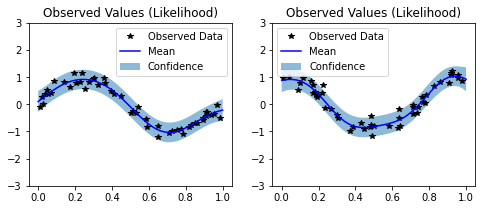
# Define plotting function
def ax_plot(ax, train_y, train_x, rand_var, title):
# Get lower and upper confidence bounds
lower, upper = rand_var.confidence_region()
# Plot training data as black stars
ax.plot(train_x.detach().numpy(), train_y.detach().numpy(), 'k*')
# Predictive mean as blue line
ax.plot(test_x.detach().numpy(), rand_var.mean.detach().numpy(), 'b')
# Shade in confidence
ax.fill_between(test_x.detach().numpy(), lower.detach().numpy(), upper.detach().numpy(), alpha=0.5)
ax.set_ylim([-3, 3])
ax.legend(['Observed Data', 'Mean', 'Confidence'])
ax.set_title(title)
# Plot both tasks
ax_plot(y1_ax, train_y1, train_x1, observed_pred_y1, 'Observed Values (Likelihood)')
ax_plot(y2_ax, train_y2, train_x2, observed_pred_y2, 'Observed Values (Likelihood)')