GPyTorch Regression Tutorial (GPU)
(This notebook is the same as the simple GP regression tutorial notebook, but does all computations on a GPU for acceleration. Check out the multi-GPU tutorial if you have large datasets that needs multiple GPUs!)
Introduction
In this notebook, we demonstrate many of the design features of GPyTorch using the simplest example, training an RBF kernel Gaussian process on a simple function. We’ll be modeling the function
with 11 training examples, and testing on 51 test examples.
[1]:
import math
import torch
import gpytorch
from matplotlib import pyplot as plt

%matplotlib inline
%load_ext autoreload
%autoreload 2
Set up training data
In the next cell, we set up the training data for this example. We’ll be using 11 regularly spaced points on [0,1] which we evaluate the function on and add Gaussian noise to get the training labels.
[2]:
# Training data is 11 points in [0,1] inclusive regularly spaced
train_x = torch.linspace(0, 1, 100)
# True function is sin(2*pi*x) with Gaussian noise
train_y = torch.sin(train_x * (2 * math.pi)) + torch.randn(train_x.size()) * 0.2
Setting up the model
See the simple GP regression tutorial for a detailed explanation for all the terms.
[3]:
class ExactGPModel(gpytorch.models.ExactGP):
    def __init__(self, train_x, train_y, likelihood):
        super(ExactGPModel, self).__init__(train_x, train_y, likelihood)
        self.mean_module = gpytorch.means.ConstantMean()
        self.covar_module = gpytorch.kernels.ScaleKernel(gpytorch.kernels.RBFKernel())

    def forward(self, x):
        mean_x = self.mean_module(x)
        covar_x = self.covar_module(x)
        return gpytorch.distributions.MultivariateNormal(mean_x, covar_x)

# initialize likelihood and model
likelihood = gpytorch.likelihoods.GaussianLikelihood()
model = ExactGPModel(train_x, train_y, likelihood)
Using the GPU
To do computations on the GPU, we need to put our data and model onto the GPU. (This requires PyTorch with CUDA).
[4]:
train_x = train_x.cuda()
train_y = train_y.cuda()
model = model.cuda()
likelihood = likelihood.cuda()
That’s it! All the training code is the same as in the simple GP regression tutorial.
Training the model
[5]:
# Find optimal model hyperparameters
model.train()
likelihood.train()

# Use the adam optimizer
optimizer = torch.optim.Adam(model.parameters(), lr=0.1)  # Includes GaussianLikelihood parameters

# "Loss" for GPs - the marginal log likelihood
mll = gpytorch.mlls.ExactMarginalLogLikelihood(likelihood, model)

training_iter = 50
for i in range(training_iter):
    # Zero gradients from previous iteration
    optimizer.zero_grad()
    # Output from model
    output = model(train_x)
    # Calc loss and backprop gradients
    loss = -mll(output, train_y)
    loss.backward()
    print('Iter %d/%d - Loss: %.3f   lengthscale: %.3f   noise: %.3f' % (
        i + 1, training_iter, loss.item(),
        model.covar_module.base_kernel.lengthscale.item(),
        model.likelihood.noise.item()
    ))
    optimizer.step()
Iter 1/50 - Loss: 0.944   lengthscale: 0.693   noise: 0.693
Iter 2/50 - Loss: 0.913   lengthscale: 0.644   noise: 0.644
Iter 3/50 - Loss: 0.879   lengthscale: 0.598   noise: 0.598
Iter 4/50 - Loss: 0.841   lengthscale: 0.555   noise: 0.554
Iter 5/50 - Loss: 0.798   lengthscale: 0.514   noise: 0.513
Iter 6/50 - Loss: 0.750   lengthscale: 0.475   noise: 0.474
Iter 7/50 - Loss: 0.698   lengthscale: 0.439   noise: 0.437
Iter 8/50 - Loss: 0.645   lengthscale: 0.405   noise: 0.402
Iter 9/50 - Loss: 0.595   lengthscale: 0.372   noise: 0.369
Iter 10/50 - Loss: 0.548   lengthscale: 0.342   noise: 0.339
Iter 11/50 - Loss: 0.507   lengthscale: 0.315   noise: 0.310
Iter 12/50 - Loss: 0.469   lengthscale: 0.292   noise: 0.284
Iter 13/50 - Loss: 0.432   lengthscale: 0.272   noise: 0.259
Iter 14/50 - Loss: 0.398   lengthscale: 0.255   noise: 0.236
Iter 15/50 - Loss: 0.363   lengthscale: 0.241   noise: 0.215
Iter 16/50 - Loss: 0.329   lengthscale: 0.230   noise: 0.196
Iter 17/50 - Loss: 0.296   lengthscale: 0.222   noise: 0.178
Iter 18/50 - Loss: 0.263   lengthscale: 0.215   noise: 0.162
Iter 19/50 - Loss: 0.230   lengthscale: 0.210   noise: 0.147
Iter 20/50 - Loss: 0.198   lengthscale: 0.207   noise: 0.134
Iter 21/50 - Loss: 0.167   lengthscale: 0.205   noise: 0.122
Iter 22/50 - Loss: 0.136   lengthscale: 0.205   noise: 0.110
Iter 23/50 - Loss: 0.107   lengthscale: 0.206   noise: 0.100
Iter 24/50 - Loss: 0.079   lengthscale: 0.208   noise: 0.091
Iter 25/50 - Loss: 0.053   lengthscale: 0.211   noise: 0.083
Iter 26/50 - Loss: 0.028   lengthscale: 0.215   noise: 0.076
Iter 27/50 - Loss: 0.006   lengthscale: 0.220   noise: 0.069
Iter 28/50 - Loss: -0.013   lengthscale: 0.225   noise: 0.063
Iter 29/50 - Loss: -0.029   lengthscale: 0.231   noise: 0.058
Iter 30/50 - Loss: -0.043   lengthscale: 0.237   noise: 0.053
Iter 31/50 - Loss: -0.053   lengthscale: 0.243   noise: 0.049
Iter 32/50 - Loss: -0.060   lengthscale: 0.249   noise: 0.045
Iter 33/50 - Loss: -0.065   lengthscale: 0.254   noise: 0.042
Iter 34/50 - Loss: -0.066   lengthscale: 0.259   noise: 0.039
Iter 35/50 - Loss: -0.066   lengthscale: 0.262   noise: 0.037
Iter 36/50 - Loss: -0.063   lengthscale: 0.265   noise: 0.035
Iter 37/50 - Loss: -0.060   lengthscale: 0.266   noise: 0.033
Iter 38/50 - Loss: -0.056   lengthscale: 0.266   noise: 0.032
Iter 39/50 - Loss: -0.052   lengthscale: 0.265   noise: 0.031
Iter 40/50 - Loss: -0.049   lengthscale: 0.262   noise: 0.030
Iter 41/50 - Loss: -0.047   lengthscale: 0.259   noise: 0.029
Iter 42/50 - Loss: -0.046   lengthscale: 0.254   noise: 0.029
Iter 43/50 - Loss: -0.046   lengthscale: 0.249   noise: 0.029
Iter 44/50 - Loss: -0.047   lengthscale: 0.243   noise: 0.029
Iter 45/50 - Loss: -0.049   lengthscale: 0.237   noise: 0.029
Iter 46/50 - Loss: -0.051   lengthscale: 0.231   noise: 0.029
Iter 47/50 - Loss: -0.054   lengthscale: 0.225   noise: 0.030
Iter 48/50 - Loss: -0.057   lengthscale: 0.219   noise: 0.030
Iter 49/50 - Loss: -0.059   lengthscale: 0.214   noise: 0.031
Iter 50/50 - Loss: -0.061   lengthscale: 0.210   noise: 0.032
Make predictions with the model
First, we need to make some test data, and then throw it onto the GPU
[6]:
test_x = torch.linspace(0, 1, 51).cuda()
Now the rest of the code follows the simple GP regression tutorial.
[7]:
# Get into evaluation (predictive posterior) mode
model.eval()
likelihood.eval()

# Test points are regularly spaced along [0,1]
# Make predictions by feeding model through likelihood
with torch.no_grad(), gpytorch.settings.fast_pred_var():
    observed_pred = likelihood(model(test_x))
    mean = observed_pred.mean
    lower, upper = observed_pred.confidence_region()
For plotting, we’re going to grab the data from the GPU and put it back on the CPU. We can accomplish this with the .cpu() function.
[8]:
mean = mean.cpu()
lower = lower.cpu()
upper = upper.cpu()

train_x = train_x.cpu()
train_y = train_y.cpu()
test_x = test_x.cpu()
[9]:
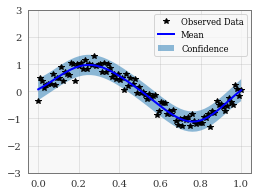
with torch.no_grad():
    # Initialize plot
    f, ax = plt.subplots(1, 1, figsize=(4, 3))

    # Plot training data as black stars
    ax.plot(train_x.numpy(), train_y.numpy(), 'k*')
    # Plot predictive means as blue line
    ax.plot(test_x.numpy(), mean.numpy(), 'b')
    # Shade between the lower and upper confidence bounds
    ax.fill_between(test_x.numpy(), lower.numpy(), upper.numpy(), alpha=0.5)
    ax.set_ylim([-3, 3])
    ax.legend(['Observed Data', 'Mean', 'Confidence'])