Metrics in GPyTorch

In this notebook, we will see how to evaluate GPyTorch models with probabilistic metrics.

Note: It is encouraged to check the Simple GP Regression notebook first if not done already. We’ll reuse most of the code from there.

We’ll be modeling the function

\[\begin{split}\begin{align} y &= \sin(2\pi x) + \epsilon \\ \epsilon &\sim \mathcal{N}(0, 0.04) \end{align}\end{split}\]

import math
import torch
import gpytorch
from matplotlib import pyplot as plt

%matplotlib inline
%load_ext autoreload
%autoreload 2

The autoreload extension is already loaded. To reload it, use:
  %reload_ext autoreload

In the next cell, we set up the train and test data.

# Training data is 100 points in [0,1] inclusive regularly spaced
train_x = torch.linspace(0, 1, 100)
# True function is sin(2*pi*x) with Gaussian noise
train_y = torch.sin(train_x * (2 * math.pi)) + torch.randn(train_x.size()) * math.sqrt(0.04)

test_x = torch.linspace(0, 1, 51)
test_y = torch.sin(test_x * (2 * math.pi)) + torch.randn(test_x.size()) * math.sqrt(0.04)

In the next cell, we define a simple GP regression model.

# We will use the simplest form of GP model, exact inference
class ExactGPModel(gpytorch.models.ExactGP):
    def __init__(self, train_x, train_y, likelihood):
        super(ExactGPModel, self).__init__(train_x, train_y, likelihood)
        self.mean_module = gpytorch.means.ConstantMean()
        self.covar_module = gpytorch.kernels.ScaleKernel(gpytorch.kernels.RBFKernel())

    def forward(self, x):
        mean_x = self.mean_module(x)
        covar_x = self.covar_module(x)
        return gpytorch.distributions.MultivariateNormal(mean_x, covar_x)

# initialize likelihood and model
likelihood = gpytorch.likelihoods.GaussianLikelihood()
model = ExactGPModel(train_x, train_y, likelihood)

Our model is ready for hyperparameter learning, but, first let us check how it performs on the test data.

model.eval()
with torch.no_grad():
    untrained_pred_dist = likelihood(model(test_x))
    predictive_mean = untrained_pred_dist.mean
    lower, upper = untrained_pred_dist.confidence_region()

f, ax = plt.subplots(1, 1, figsize=(4, 3))
# Plot training data as black stars
ax.plot(train_x, train_y, 'k*')
# Plot predictive means as blue line
ax.plot(test_x, predictive_mean, 'b')
# Shade between the lower and upper confidence bounds
ax.fill_between(test_x, lower, upper, alpha=0.5)
ax.set_ylim([-3, 3])
ax.legend(['Observed Data', 'Mean', 'Confidence'], bbox_to_anchor=(1.6,1));

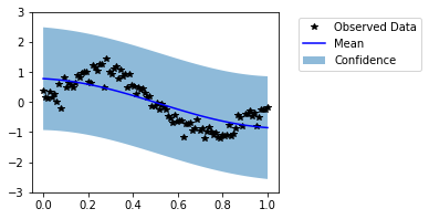
Visually, this does not look like a good fit. Now, let us train the model hyperparameters.

# this is for running the notebook in our testing framework
import os
smoke_test = ('CI' in os.environ)
training_iter = 2 if smoke_test else 50


# Find optimal model hyperparameters
model.train()

# Use the adam optimizer
optimizer = torch.optim.Adam(model.parameters(), lr=0.1)  # Includes GaussianLikelihood parameters

# "Loss" for GPs - the marginal log likelihood
mll = gpytorch.mlls.ExactMarginalLogLikelihood(likelihood, model)

for i in range(training_iter):
    # Zero gradients from previous iteration
    optimizer.zero_grad()
    # Output from model
    output = model(train_x)
    # Calc loss and backprop gradients
    loss = -mll(output, train_y)
    loss.backward()
    print('Iter %d/%d - Loss: %.3f   lengthscale: %.3f   noise: %.3f' % (
        i + 1, training_iter, loss.item(),
        model.covar_module.base_kernel.lengthscale.item(),
        model.likelihood.noise.item()
    ))
    optimizer.step()

Iter 1/50 - Loss: 0.944   lengthscale: 0.693   noise: 0.693
Iter 2/50 - Loss: 0.913   lengthscale: 0.644   noise: 0.644
Iter 3/50 - Loss: 0.879   lengthscale: 0.598   noise: 0.598
Iter 4/50 - Loss: 0.841   lengthscale: 0.555   noise: 0.554
Iter 5/50 - Loss: 0.798   lengthscale: 0.514   noise: 0.513
Iter 6/50 - Loss: 0.750   lengthscale: 0.475   noise: 0.474
Iter 7/50 - Loss: 0.698   lengthscale: 0.439   noise: 0.437
Iter 8/50 - Loss: 0.645   lengthscale: 0.404   noise: 0.402
Iter 9/50 - Loss: 0.594   lengthscale: 0.372   noise: 0.369
Iter 10/50 - Loss: 0.547   lengthscale: 0.342   noise: 0.339
Iter 11/50 - Loss: 0.505   lengthscale: 0.315   noise: 0.310
Iter 12/50 - Loss: 0.466   lengthscale: 0.291   noise: 0.284
Iter 13/50 - Loss: 0.430   lengthscale: 0.271   noise: 0.259
Iter 14/50 - Loss: 0.395   lengthscale: 0.254   noise: 0.236
Iter 15/50 - Loss: 0.361   lengthscale: 0.240   noise: 0.215
Iter 16/50 - Loss: 0.327   lengthscale: 0.229   noise: 0.196
Iter 17/50 - Loss: 0.294   lengthscale: 0.220   noise: 0.178
Iter 18/50 - Loss: 0.261   lengthscale: 0.214   noise: 0.162
Iter 19/50 - Loss: 0.228   lengthscale: 0.209   noise: 0.147
Iter 20/50 - Loss: 0.196   lengthscale: 0.206   noise: 0.134
Iter 21/50 - Loss: 0.164   lengthscale: 0.205   noise: 0.122
Iter 22/50 - Loss: 0.133   lengthscale: 0.204   noise: 0.110
Iter 23/50 - Loss: 0.104   lengthscale: 0.205   noise: 0.100
Iter 24/50 - Loss: 0.076   lengthscale: 0.207   noise: 0.091
Iter 25/50 - Loss: 0.049   lengthscale: 0.210   noise: 0.083
Iter 26/50 - Loss: 0.025   lengthscale: 0.214   noise: 0.076
Iter 27/50 - Loss: 0.003   lengthscale: 0.218   noise: 0.069
Iter 28/50 - Loss: -0.017   lengthscale: 0.223   noise: 0.063
Iter 29/50 - Loss: -0.033   lengthscale: 0.228   noise: 0.058
Iter 30/50 - Loss: -0.047   lengthscale: 0.233   noise: 0.053
Iter 31/50 - Loss: -0.057   lengthscale: 0.239   noise: 0.049
Iter 32/50 - Loss: -0.065   lengthscale: 0.243   noise: 0.045
Iter 33/50 - Loss: -0.069   lengthscale: 0.248   noise: 0.042
Iter 34/50 - Loss: -0.071   lengthscale: 0.252   noise: 0.039
Iter 35/50 - Loss: -0.071   lengthscale: 0.255   noise: 0.037
Iter 36/50 - Loss: -0.069   lengthscale: 0.257   noise: 0.035
Iter 37/50 - Loss: -0.066   lengthscale: 0.257   noise: 0.033
Iter 38/50 - Loss: -0.062   lengthscale: 0.257   noise: 0.032
Iter 39/50 - Loss: -0.058   lengthscale: 0.255   noise: 0.031
Iter 40/50 - Loss: -0.055   lengthscale: 0.252   noise: 0.030
Iter 41/50 - Loss: -0.054   lengthscale: 0.248   noise: 0.029
Iter 42/50 - Loss: -0.053   lengthscale: 0.243   noise: 0.029
Iter 43/50 - Loss: -0.053   lengthscale: 0.237   noise: 0.029
Iter 44/50 - Loss: -0.055   lengthscale: 0.230   noise: 0.029
Iter 45/50 - Loss: -0.057   lengthscale: 0.223   noise: 0.029
Iter 46/50 - Loss: -0.060   lengthscale: 0.216   noise: 0.029
Iter 47/50 - Loss: -0.063   lengthscale: 0.208   noise: 0.030
Iter 48/50 - Loss: -0.066   lengthscale: 0.202   noise: 0.030
Iter 49/50 - Loss: -0.068   lengthscale: 0.196   noise: 0.031
Iter 50/50 - Loss: -0.070   lengthscale: 0.190   noise: 0.032

In the next cell, we reevaluate the model on the test data.

model.eval()
with torch.no_grad():
    trained_pred_dist = likelihood(model(test_x))
    predictive_mean = trained_pred_dist.mean
    lower, upper = trained_pred_dist.confidence_region()

f, ax = plt.subplots(1, 1, figsize=(4, 3))
# Plot training data as black stars
ax.plot(train_x, train_y, 'k*')
# Plot predictive means as blue line
ax.plot(test_x, predictive_mean, 'b')
# Shade between the lower and upper confidence bounds
ax.fill_between(test_x, lower, upper, alpha=0.5)
ax.set_ylim([-3, 3])
ax.legend(['Observed Data', 'Mean', 'Confidence'], bbox_to_anchor=(1.6,1));

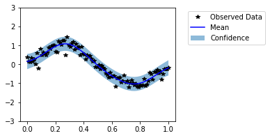
Now our model seems to fit well on the data. It is not always possible to visually evaluate the model in high dimensional cases. Thus, now we evaluate the models with help of probabilistic metrics. We have saved predictive distributions from untrained and trained models as untrained_pred_dist and trained_pred_dist respectively.

Negative Log Predictive Density (NLPD)

Negative Log Predictive Density (NLPD) is the most standard probabilistic metric for evaluating GP models. In simple terms, it is negative log likelihood of the test data given the predictive distribution. It can be computed as follows:

init_nlpd = gpytorch.metrics.negative_log_predictive_density(untrained_pred_dist, test_y)
final_nlpd = gpytorch.metrics.negative_log_predictive_density(trained_pred_dist, test_y)

print(f'Untrained model NLPD: {init_nlpd:.2f}, \nTrained model NLPD: {final_nlpd:.2f}')

Untrained model NLPD: 0.88,
Trained model NLPD: -0.21

Mean Standardized Log Loss (MSLL)

This metric computes average negative log likelihood of all test points w.r.t their univariate predicitve densities. For more details, see “page No. 23, Gaussian Processes for Machine Learning, Carl Edward Rasmussen and Christopher K. I. Williams, The MIT Press, 2006. ISBN 0-262-18253-X”

init_msll = gpytorch.metrics.mean_standardized_log_loss(untrained_pred_dist, test_y)
final_msll = gpytorch.metrics.mean_standardized_log_loss(trained_pred_dist, test_y)

print(f'Untrained model MSLL: {init_msll:.2f}, \nTrained model MSLL: {final_msll:.2f}')

Untrained model MSLL: 0.82,
Trained model MSLL: -0.49

It is also possible to calculate the quantile coverage error with gpytorch.metrics.quantile_coverage_error function.

quantile = 95
qce = gpytorch.metrics.quantile_coverage_error(trained_pred_dist, test_y, quantile=quantile)
print(f'Quantile {quantile}% Coverage Error: {qce:.2f}')

Quantile 95% Coverage Error: 0.01

Mean Squared Error (MSE)

Mean Squared Error (MSE) is the mean of the squared difference between the test observations and the predictive mean. It is a well-known conventional metric for evaluating regression models. However, it can not take uncertainty into account unlike NLPD, MLSS and ACE.

init_mse = gpytorch.metrics.mean_squared_error(untrained_pred_dist, test_y, squared=True)
final_mse = gpytorch.metrics.mean_squared_error(trained_pred_dist, test_y, squared=True)

print(f'Untrained model MSE: {init_mse:.2f}, \nTrained model MSE: {final_mse:.2f}')

Untrained model MSE: 0.20,
Trained model MSE: 0.04

Mean Absolute Error (MAE)

Mean Absolute Error (MAE) is the mean of the absolute difference between the test observations and the predictive mean. It is less sensitive to the outliers than MSE.

init_mae = gpytorch.metrics.mean_absolute_error(untrained_pred_dist, test_y)
final_mae = gpytorch.metrics.mean_absolute_error(trained_pred_dist, test_y)

print(f'Untrained model MAE: {init_mae:.2f}, \nTrained model MAE: {final_mae:.2f}')

Untrained model MAE: 0.38,
Trained model MSE: 0.16