Spectral GP Learning with Deltas

In this paper, we demonstrate another approach to spectral learning with GPs, learning a spectral density as a simple mixture of deltas. This has been explored, for example, as early as Lázaro-Gredilla et al., 2010.

Compared to learning Gaussian mixtures as in the SM kernel, this approach has a number of pros and cons. In its favor, it is often very robust and does not have as severe issues with local optima, as it is easier to make progress when performing gradient descent on 1 of 1000 deltas compared to the parameters of 1 of 3 Gaussians. Additionally, implemented using CG in GPyTorch, this approach affords linear time and space in the number of data points N. Against it, it has significantly more parameters which can take many more iterations of training to learn, and it corresponds to a finite basis expansion and is therefore a parametric model.

import gpytorch
import torch

Load Data

For this notebook, we’ll be using a sample set of timeseries data of BART ridership on the 5 most commonly traveled stations in San Francisco. This subsample of data was selected and processed from Pyro’s examples http://docs.pyro.ai/en/stable/_modules/pyro/contrib/examples/bart.html

import os
import urllib.request

smoke_test = ('CI' in os.environ)

if not smoke_test and not os.path.isfile('../BART_sample.pt'):
    print('Downloading \'BART\' sample dataset...')
    urllib.request.urlretrieve('https://drive.google.com/uc?export=download&id=1A6LqCHPA5lHa5S3lMH8mLMNEgeku8lRG', '../BART_sample.pt')
    torch.manual_seed(1)

if smoke_test:
    train_x, train_y, test_x, test_y = torch.randn(2, 100, 1), torch.randn(2, 100), torch.randn(2, 100, 1), torch.randn(2, 100)
else:
    train_x, train_y, test_x, test_y = torch.load('../BART_sample.pt', map_location='cpu')

if torch.cuda.is_available():
    train_x, train_y, test_x, test_y = train_x.cuda(), train_y.cuda(), test_x.cuda(), test_y.cuda()

print(train_x.shape, train_y.shape, test_x.shape, test_y.shape)

torch.Size([5, 1440, 1]) torch.Size([5, 1440]) torch.Size([5, 240, 1]) torch.Size([5, 240])

train_x_min = train_x.min()
train_x_max = train_x.max()

train_x = train_x - train_x_min
test_x = test_x - train_x_min

train_y_mean = train_y.mean(dim=-1, keepdim=True)
train_y_std = train_y.std(dim=-1, keepdim=True)

train_y = (train_y - train_y_mean) / train_y_std

test_y = (test_y - train_y_mean) / train_y_std

Define a Model

The only thing of note here is the use of the kernel. For this example, we’ll learn a kernel with 2048 deltas in the mixture, and initialize by sampling directly from the empirical spectrum of the data.

class SpectralDeltaGP(gpytorch.models.ExactGP):
    def __init__(self, train_x, train_y, num_deltas, noise_init=None):
        likelihood = gpytorch.likelihoods.GaussianLikelihood(noise_constraint=gpytorch.constraints.GreaterThan(1e-11))
        likelihood.register_prior("noise_prior", gpytorch.priors.HorseshoePrior(0.1), "noise")
        likelihood.noise = 1e-2

        super(SpectralDeltaGP, self).__init__(train_x, train_y, likelihood)
        self.mean_module = gpytorch.means.ConstantMean()
        base_covar_module = gpytorch.kernels.SpectralDeltaKernel(
            num_dims=train_x.size(-1),
            num_deltas=num_deltas,
        )
        base_covar_module.initialize_from_data(train_x[0], train_y[0])
        self.covar_module = gpytorch.kernels.ScaleKernel(base_covar_module)

    def forward(self, x):
        mean_x = self.mean_module(x)
        covar_x = self.covar_module(x)
        return gpytorch.distributions.MultivariateNormal(mean_x, covar_x)

model = SpectralDeltaGP(train_x, train_y, num_deltas=1500)

if torch.cuda.is_available():
    model = model.cuda()

Train

model.train()
mll = gpytorch.mlls.ExactMarginalLogLikelihood(model.likelihood, model)
optimizer = torch.optim.Adam(model.parameters(), lr=0.01)
scheduler = torch.optim.lr_scheduler.MultiStepLR(optimizer=optimizer, milestones=[40])

num_iters = 1000 if not smoke_test else 4

with gpytorch.settings.max_cholesky_size(0):  # Ensure we dont try to use Cholesky
    for i in range(num_iters):
        optimizer.zero_grad()
        output = model(train_x)
        loss = -mll(output, train_y)
        if train_x.dim() == 3:
            loss = loss.mean()
        loss.backward()
        optimizer.step()

        if i % 10 == 0:
            print(f'Iteration {i} - loss = {loss:.2f} - noise = {model.likelihood.noise.item():e}')

        scheduler.step()

Iteration 0 - loss = 24.75 - noise = 1.010000e-02
Iteration 10 - loss = 10.49 - noise = 1.107906e-02
Iteration 20 - loss = 3.68 - noise = 1.204213e-02
Iteration 30 - loss = 3.69 - noise = 1.276487e-02
Iteration 40 - loss = 2.00 - noise = 1.333853e-02
Iteration 50 - loss = 1.18 - noise = 1.337870e-02
Iteration 60 - loss = 1.10 - noise = 1.340098e-02
Iteration 70 - loss = 1.06 - noise = 1.341575e-02
Iteration 80 - loss = 1.05 - noise = 1.342753e-02
Iteration 90 - loss = 0.98 - noise = 1.343861e-02
Iteration 100 - loss = 0.98 - noise = 1.344975e-02
Iteration 110 - loss = 0.91 - noise = 1.346152e-02
Iteration 120 - loss = 0.94 - noise = 1.347341e-02
Iteration 130 - loss = 0.90 - noise = 1.348564e-02
Iteration 140 - loss = 0.78 - noise = 1.349751e-02
Iteration 150 - loss = 0.75 - noise = 1.350786e-02
Iteration 160 - loss = 0.75 - noise = 1.351690e-02
Iteration 170 - loss = 0.76 - noise = 1.352605e-02
Iteration 180 - loss = 0.74 - noise = 1.353530e-02
Iteration 190 - loss = 0.71 - noise = 1.354463e-02
Iteration 200 - loss = 0.71 - noise = 1.355418e-02
Iteration 210 - loss = 0.71 - noise = 1.356385e-02
Iteration 220 - loss = 0.71 - noise = 1.357375e-02
Iteration 230 - loss = 0.71 - noise = 1.358384e-02
Iteration 240 - loss = 0.70 - noise = 1.359454e-02
Iteration 250 - loss = 0.65 - noise = 1.360544e-02
Iteration 260 - loss = 0.69 - noise = 1.361629e-02
Iteration 270 - loss = 0.68 - noise = 1.362717e-02
Iteration 280 - loss = 0.67 - noise = 1.363807e-02
Iteration 290 - loss = 0.70 - noise = 1.364926e-02
Iteration 300 - loss = 0.70 - noise = 1.366061e-02
Iteration 310 - loss = 0.66 - noise = 1.367212e-02
Iteration 320 - loss = 0.65 - noise = 1.368315e-02
Iteration 330 - loss = 0.65 - noise = 1.369375e-02
Iteration 340 - loss = 0.64 - noise = 1.370386e-02
Iteration 350 - loss = 0.64 - noise = 1.371405e-02
Iteration 360 - loss = 0.62 - noise = 1.372444e-02
Iteration 370 - loss = 0.63 - noise = 1.373496e-02
Iteration 380 - loss = 0.63 - noise = 1.374584e-02
Iteration 390 - loss = 0.63 - noise = 1.375700e-02
Iteration 400 - loss = 0.63 - noise = 1.376797e-02
Iteration 410 - loss = 0.60 - noise = 1.377904e-02
Iteration 420 - loss = 0.61 - noise = 1.379027e-02
Iteration 430 - loss = 0.61 - noise = 1.380114e-02
Iteration 440 - loss = 0.62 - noise = 1.381227e-02
Iteration 450 - loss = 0.61 - noise = 1.382362e-02
Iteration 460 - loss = 0.58 - noise = 1.383517e-02
Iteration 470 - loss = 0.61 - noise = 1.384682e-02
Iteration 480 - loss = 0.63 - noise = 1.385889e-02
Iteration 490 - loss = 0.63 - noise = 1.387111e-02
Iteration 500 - loss = 0.61 - noise = 1.388358e-02
Iteration 510 - loss = 0.60 - noise = 1.389664e-02
Iteration 520 - loss = 0.60 - noise = 1.390998e-02
Iteration 530 - loss = 0.58 - noise = 1.392351e-02
Iteration 540 - loss = 0.62 - noise = 1.393629e-02
Iteration 550 - loss = 0.60 - noise = 1.394872e-02
Iteration 560 - loss = 0.60 - noise = 1.396085e-02
Iteration 570 - loss = 0.59 - noise = 1.397342e-02
Iteration 580 - loss = 0.63 - noise = 1.398654e-02
Iteration 590 - loss = 0.58 - noise = 1.400001e-02
Iteration 600 - loss = 0.58 - noise = 1.401340e-02
Iteration 610 - loss = 0.62 - noise = 1.402742e-02
Iteration 620 - loss = 0.59 - noise = 1.404199e-02
Iteration 630 - loss = 0.63 - noise = 1.405650e-02
Iteration 640 - loss = 0.63 - noise = 1.407137e-02
Iteration 650 - loss = 0.60 - noise = 1.408640e-02
Iteration 660 - loss = 0.58 - noise = 1.410100e-02
Iteration 670 - loss = 0.61 - noise = 1.411567e-02
Iteration 680 - loss = 0.59 - noise = 1.413125e-02
Iteration 690 - loss = 0.61 - noise = 1.414781e-02
Iteration 700 - loss = 0.58 - noise = 1.416490e-02
Iteration 710 - loss = 0.59 - noise = 1.418221e-02
Iteration 720 - loss = 0.59 - noise = 1.420006e-02
Iteration 730 - loss = 0.60 - noise = 1.421693e-02
Iteration 740 - loss = 0.59 - noise = 1.423384e-02
Iteration 750 - loss = 0.59 - noise = 1.424886e-02
Iteration 760 - loss = 0.59 - noise = 1.426466e-02
Iteration 770 - loss = 0.58 - noise = 1.428063e-02
Iteration 780 - loss = 0.60 - noise = 1.429628e-02
Iteration 790 - loss = 0.62 - noise = 1.431342e-02
Iteration 800 - loss = 0.57 - noise = 1.433162e-02
Iteration 810 - loss = 0.61 - noise = 1.435035e-02
Iteration 820 - loss = 0.57 - noise = 1.436906e-02
Iteration 830 - loss = 0.58 - noise = 1.438674e-02
Iteration 840 - loss = 0.58 - noise = 1.440415e-02
Iteration 850 - loss = 0.61 - noise = 1.442217e-02
Iteration 860 - loss = 0.58 - noise = 1.444128e-02
Iteration 870 - loss = 0.59 - noise = 1.445954e-02
Iteration 880 - loss = 0.61 - noise = 1.447739e-02
Iteration 890 - loss = 0.58 - noise = 1.449536e-02
Iteration 900 - loss = 0.54 - noise = 1.451268e-02
Iteration 910 - loss = 0.54 - noise = 1.452836e-02
Iteration 920 - loss = 0.55 - noise = 1.454423e-02
Iteration 930 - loss = 0.59 - noise = 1.456236e-02
Iteration 940 - loss = 0.56 - noise = 1.457988e-02
Iteration 950 - loss = 0.57 - noise = 1.459668e-02
Iteration 960 - loss = 0.56 - noise = 1.461400e-02
Iteration 970 - loss = 0.47 - noise = 1.462959e-02
Iteration 980 - loss = 0.47 - noise = 1.464033e-02
Iteration 990 - loss = 0.46 - noise = 1.464958e-02

# Get into evaluation (predictive posterior) mode
model.eval()

# Test points are regularly spaced along [0,1]
# Make predictions by feeding model through likelihood
with torch.no_grad(), gpytorch.settings.max_cholesky_size(0), gpytorch.settings.fast_pred_var():
    test_x_f = torch.cat([train_x, test_x], dim=-2)
    observed_pred = model.likelihood(model(test_x_f))
    varz = observed_pred.variance

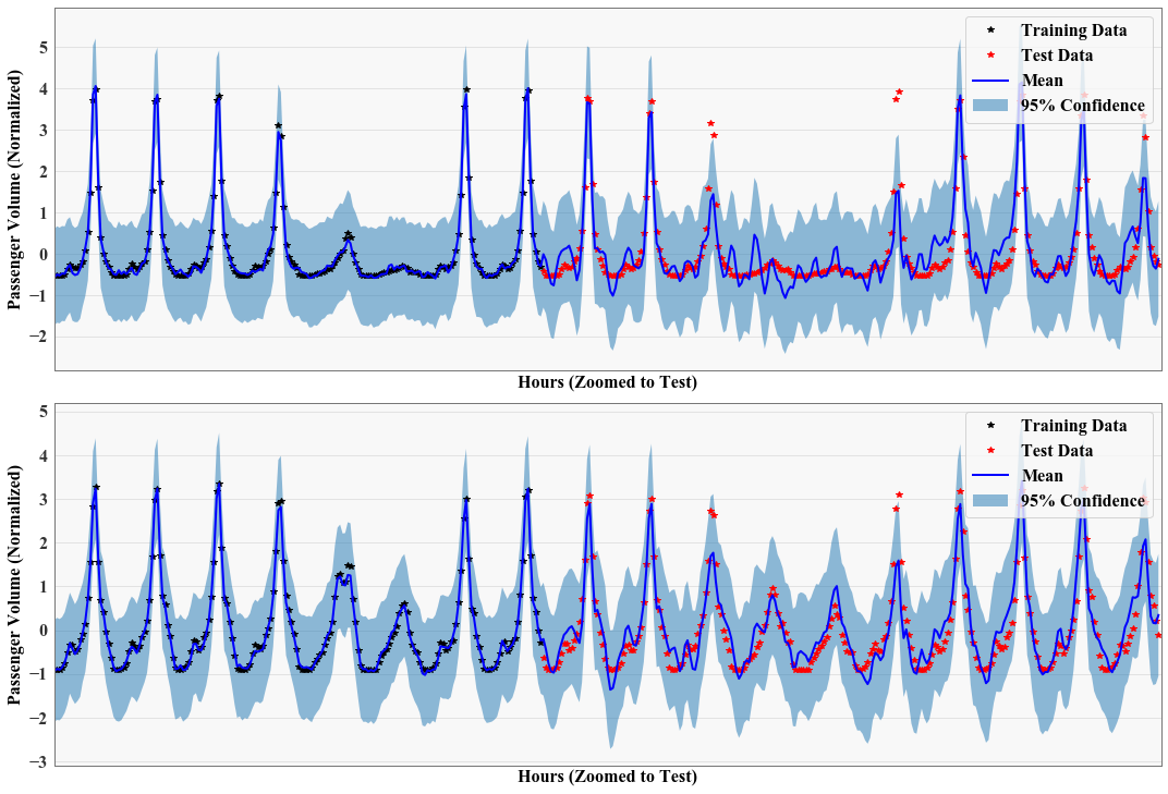
Plot Results

from matplotlib import pyplot as plt

%matplotlib inline

_task = 3

plt.subplots(figsize=(15, 15), sharex=True, sharey=True)
for _task in range(2):
    ax = plt.subplot(3, 1, _task + 1)

    with torch.no_grad():
        # Initialize plot
#         f, ax = plt.subplots(1, 1, figsize=(16, 12))

        # Get upper and lower confidence bounds
        lower = observed_pred.mean - varz.sqrt() * 1.98
        upper = observed_pred.mean + varz.sqrt() * 1.98
        lower = lower[_task] #  + weight * test_x_f.squeeze()
        upper = upper[_task] # + weight * test_x_f.squeeze()

        # Plot training data as black stars
        ax.plot(train_x[_task].detach().cpu().numpy(), train_y[_task].detach().cpu().numpy(), 'k*')
        ax.plot(test_x[_task].detach().cpu().numpy(), test_y[_task].detach().cpu().numpy(), 'r*')
        # Plot predictive means as blue line
        ax.plot(test_x_f[_task].detach().cpu().numpy(), (observed_pred.mean[_task]).detach().cpu().numpy(), 'b')
        # Shade between the lower and upper confidence bounds
        ax.fill_between(test_x_f[_task].detach().cpu().squeeze().numpy(), lower.detach().cpu().numpy(), upper.detach().cpu().numpy(), alpha=0.5)
    #     ax.set_ylim([-3, 3])
        ax.legend(['Training Data', 'Test Data', 'Mean', '95% Confidence'], fontsize=16)
        ax.tick_params(axis='both', which='major', labelsize=16)
        ax.tick_params(axis='both', which='minor', labelsize=16)
        ax.set_ylabel('Passenger Volume (Normalized)', fontsize=16)
        ax.set_xlabel('Hours (Zoomed to Test)', fontsize=16)
        ax.set_xticks([])

        plt.xlim([1250, 1680])

plt.tight_layout()